Studies in Quality Improvement: Designing Environmental Regulations

CQPI Report No. 7
Søren Bisgaard and William G. Hunter
Copyright © February 1986, Used by permission

This research was supported in part by grants SES - 8018418 and DMS - 8420968 from the National Science Foundation and an award from the Graduate School, University of Wisconsin - Madison, through the University - Industry Research Program. Computing was facilitated by access to the research computer at the Department of Statistics, University of Wisconsin - Madison. Completed February 1986.

Practical Significance

Methods of statistical quality control have been used successfully in industry. These same methods can be applied in non - traditional contexts in which quality is to be controlled and, if possible, improved. This report considers a wider context in which industry and society exist: the environment. The quality of the environment must be protected, whether it be considered on a local, state-wide, regional, national, or international basis. One way that this problem is being handled is through the promulgation and enforcement of environmental standards by various governmental bodies.

This report explains how standards can be developed on a more rational basis so that the errors that inevitably will be made during enforcement are confronted and balanced, rather than ignored. In particular, this report outlines a framework, which is based on statistical quality control concepts, for designing environmental regulations. This framework explicitly takes into account the statistical nature of environmental data. It is shown how the operating characteristic function can be useful in designing new standards and evaluating existing standards. With slight modifications, the framework outlined in this report can be applied to the design of standards of all kinds, including industrial standards.

Keywords: Environmental standards, compliance, statistical quality control, operating characteristic function, type I and type II errors, environmental data, risk, ambient ozone, research needs.

Public debate on proposed environmental regulations often focuses almost entirely (and naively) on the allowable limit for a particular pollutant, with scant attention being paid to the statistical nature of environmental data and to the operational definition of compliance. As a consequence regulations may fail to accomplish their purpose. A unifying framework is therefore proposed that interrelates assessment of risk aid determination of compliance. A central feature is the operating characteristic curve, which displays the discriminating power of a regulation. This framework can facilitate rational discussion among scientists, policymakers, and others concerned with environmental regulation.

Introduction

Over the past twenty years many new federal, state, and local regulations have resulted from heightened concern about the damage that we humans have done to the environment - and might do in the future. Public debate, unfortunately, has often focused almost exclusively on risk assessment and the allowable limit of a pollutant. Although this "limit part" of regulation is important, a regulation also include a "statistical part" that defines how compliance is to be determined even though it is typically relegated to an appendix and thus may seem unimportant, it can have a profound effect on how the regulation performs.

Our purpose in this article is to introduce some new ideas concerning the general problem of designing environmental regulations, and, in particular, to consider the role of the "statistical part" of such regulations. As a vehicle for illustration, we use the environmental regulation of ambient ozone. Our intent is not to provide a definitive analysis of that particular problem. Indeed, that would require experts familiar with the generation, dispersion, measurements, and monitoring of ozone to analyze available data sets. Such detailed analysis would probably lead to the adoption of somewhat different statistical assumptions than we use. The methodology described below, however, can accommodate any reasonable statistical assumptions for ambient ozone. Moreover, this methodology can be used in the rational design of any environmental regulation to limit exposure to any pollutant.

Ambient Ozone Standard

For illustrative purposes, then, let us consider the ambient ozone standard (1, 2). Ozone is a reactive form of oxygen that has serious health effects. Concentrations from about 0.15 parts per million (ppm), for example, affect respiratory mucous membranes and other lung tissues in sensitive individuals as well as healthy exercising persons. In 1971, based on the best scientific studies at the time, the Environmental Protection Agency (EPA) promulgated a National Primary and Secondary Ambient Air Quality Standard ruling that "an hourly average level of 0.08 parts per million (ppm) not to be" exceeded more than 1 hour per year. Section 109(d) of the Clean Air Act calls for a review every five years of the Primary National Ambient Air Quality Standards. In 1977 EPA announced that it was reviewing and updating the 1911 ozone standard. In preparing a new criteria document, EPA provided a number of opportunities for external review and comment. Two drafts of the document were made available for external review. EPA received more than 50 written responses to the first draft and approximately 20 to the second draft. The American Petroleum Institute (API), in particular, submitted extensive comments.

The criteria document was the subject of two meetings of the Subcommittee on Scientific Criteria for Photochemical Oxidants of EPA's Science Advisory Board. At each of these meetings, which were open to the public, critical review and new information was presented for EPA's consideration. The Agency was petitioned by the API and 29 member companies and by the City of Houston around the time the revision was announced. Among other things, the petition requested that EPA state the primary and secondary standards in such a way as to permit reliable assessment of compliance. In the Federal Register it is noted that

EPA agrees that the present deterministic form standard has several limitations and has made reliable assessment of compliance difficult. The revised ozone air quality standards are stated in a statistical form that will more accurately reflect the air quality problems in various regions of the country and allow more reliable assessment of compliance with the standards. (Emphasis added).

Later, in the begging of 1978, the EPA held a public meeting to receive comments from interested parties on the initial proposed revision of the standard. Here several representatives from the State and Territorial Air Pollution Program Administrators (STAPPA) and the Association of Local Air Pollution Control Officials participated. After the proposal was published in the spring of 1978, EPA held four public meetings to receive comments on the proposed standard revisions. In addition, 168 written comments were received during the formal continent period. The Federal Register summarizes the comments as follows:

The majority of comments received (132 out of 168) opposed EPA's proposed standard revision, favoring either a more relaxed or a more stringent standard. State air pollution control agencies (and STAPPA) generally supported a standard level of 0.12 ppm on the basis of their assessment of an adequate margin of safety. Municipal groups generally supported a standard level of 0.12 ppm or higher, whereas most industrial groups supported a standard level 10.15 ppm or higher. Environmental groups generally encouraged EPA to retain the 0.08 ppm standard.

As reflected in this statement, almost all of the public discussion of the ambient ozone standard (not just the 168 comments summarized here) focused on the limit part of the regulation. In this instance, in common with similar discussion of other environmental regulations, the statistical part of the regulation was largely ignored.

The final rule-making made the following three changes:

1. The primary standard was raised to 0.12 ppm.
2. The secondary standard was raised to 0.12 ppm.
3. The definition of the point at which the standard is attained was changed to "when the expected number of days per calendar year, with maximum hourly average concentration above 0.12 ppm is equal to or less than one."

The Operating Characteristic Curve

Environmentalregulations have a structure similar to that of statistical hypothesis tests. A regulation states how data are to be used to decide whether a particular site is in compliance with a specified standard, and a hypothesis test states how a particular set of data are to be used to decide whether they are in reasonable agreement with a specified hypothesis. Borrowing the terminology and methodology from hypothesis testing, we can say there are two types of errors that can be made because of the stochastic nature of environmental data: a site that is really in compliance can be declared out of compliance (type I error) and vice versa (type II error). Ideally the probability of committing both types of error should be zero. In practice, however, it is not feasible to obtain this Ideal.

In the context of environmental regulations, an operating characteristic curve is the probability of declaring a site to be in compliance (d.i.c.) plotted as a function of some parameter θ such as the mean level of a pollutant. This Prob (d.i.c. | θ) can be used to determine the probabilities of committing type I and type II errors. As long as θ is below the stated standard, the probability of a type I error is

1 - Prob (d.i.c.| θ). When θ above the stated standard, Prob (d.i.c. | θ) is the probability of a type II error. Using the operating characteristic curve for the old and the new regulations for ambient ozone, we can evaluate them to see what was accomplished by the revision.

The old standard stated that "an hourly average level of 0.08 ppm [was] not to be exceeded more than 1 hour per year." This standard was therefore defined operationally in terms of the observations themselves. The new standard, on the other hand, states that the expected number of days per calendar year with a maximum hourly average concentration above 0.12 ppm should be less than one. Compliance, however, must be determined in terms of the actual data, not an unobserved expected number.

How should this conversion be made? In Appendix D of the new ozone regulation, it is stated that:

In general, the average number of exceedances per calendar year must be less than or equal to 1. In its simplest form, the number of exceedances at a monitoring site would be recorded for each calendar year and then averaged over the past 3 calendar years to determine if this average is less than or equal to 1.

Based on the stated requirements of compliance, we have computed the operating characteristic functions for the old and the new ozone regulations. They are plotted in Figures 1 and 2. (The last sentence in the legend for Figure 1 will be discussed below in the following section, Statistical Analysis.) To construct these curves, certain simplifying assumptions were made, which are discussed hi the section entitled "Statistical Concepts." Before such curves are used in practice, these assumptions need to be Investigated and probably modified.

According to the main part of the new ozone regulation, the interval from 0 to 1 expected number of exceedances of 0.12 ppm per year can be regarded as defining "being in compliance." Suppose the decision rule outlined above is used for a site that is operating at a level such that the expected number of days exceeding 0.12 ppm is just below one. In that case, as was noted by Javitz (3), with the new ozone regulation, there is a probability of approximately 37% in any given year that such a site will be declared out of compliance. Moreover, there is approximately a 10% chance of not detecting a violation of 2 expected days per year above the 0.12 ppm limit; that is, the standard operates such that the probability is 10% of not detecting occurrences when the actual value is twice its permissible value (2 instead of 1). Some individuals may find these probabilities (37% and 10%) to be surprisingly and unacceptably high, as we do. Others, however, may regard them as being reasonable or too low. In this paper, our point is not to pursue that particular debate. Rather, it is simply to argue that, before environmental regulations are put in place, different segments of society need to be aware of such operating characteristics, so that informed policy decisions can be made. It is important to realize that the relevant operating characteristic curves can be constructed before a regulation is promulgated.

Statical Concepts

Let X denote a measurement from an instrument such that X = θ + ε, where = θ is the mean value of the pollutant and ε is the statistical error term with variance σ². The term ε contains not only the error arising from an imperfect instrument but also the fluctuations in the level of the pollutant itself. We assume that the measurement process is well calibrated and that the mean value of ε is zero. The parameters θ and σ² of the distribution of e are unknown but estimates of them can be obtained from data. A prescription of how the data are to be collected is known as the sampling plan. It addresses the questions of how many, where, when, and how observations are to be collected. Any function ƒ(X)= ƒ(X₁, X₂, . . . ,X_n) of the observations is an estimator, for example, the average of a set of values or the number of observations in a sample above a certain limit. The value of the function f for a given sample is an estimate. The estimator has a distribution, which can be determined from the distribution of the observations and the functional form of the estimator. With the distribution of the estimator, one can answer questions of the form: what is the probability that the estimate ƒ= ƒ(X) is smaller than or equal to some critical value c? Symbolically this probability can be written as P = Prob {ƒ(X)≤c | θ}.

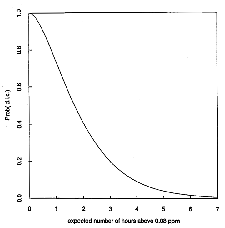
Figure 1. Operating characteristic curve for the 1971 ambient ozone standard (old standard), as a function of the expected number of hours of exceedances of 0.08 ppm per year. Note that if the old standard had been written in terms of allowable limit of one for the expected number of exceedances above 0.08 ppm, the maximum type I error would be 1.00 - 0.73 = 0.27.

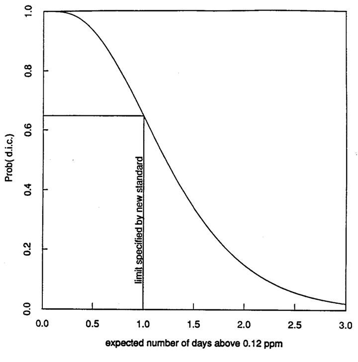
Figure 2. Operating characteristic curve for the 1979 ambient ozone standard (new standard), as a function of the expected number of days of exceedances of 0.12 ppm per year. Note that the maximum type I error is 1.00 - 0.63 = 0.37

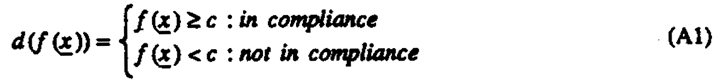
If we warn to have a regulation limiting the pollution to a certain level, it is not enough to state the limit as a particular value of a parameter. We must define compliance operationally in terms of the observations. The condition of compliance therefore takes the form of an estimator ƒ(X₁, . . . ,X_n), being less than or equal to some critical value c, that is, {ƒ (X₁, . . . ,X_n)≤ c}. Regarded as a function of θ, the probability Prob { ƒ(X_1, . . . ,X_n)≤c | θ}. is therefore the probability that the site will be declared to be in compliance with the regulation. It is, in fact, the operating characteristic function.

The operating characteristic function and consequently the probability of type I and type II errors are fixed by appropriate choice of the critical value and sampling plan. It is common statistical practice to specify a maximum type I error probability a and then to find a critical value c such that Prob {ƒ(X)≤c | θ₀} = 1 - α. To control the probability of type II errors, one would then design a sampling plan such that the probability of the type II errors is at most β for a specific value θ₁ outside the compliance region. It is important to recognize that θ₀ and c are different θ₀ is a point in the parameter space and c is a point in the sample space. Ignoring this subtle difference (which is almost always done in legal, legislative, and policymaking discussions) has led to unnecessary confusion. Because this difference exists, type I and type II errors exist. These errors should be confronted and balanced, not ignored.

Statistical Analysis

For purposes of illustration, let us consider the old and new regulations for ambient ozone. Let X denote the hourly average ozone level and let L be the limit, which for the old regulation was 0.08 ppm.

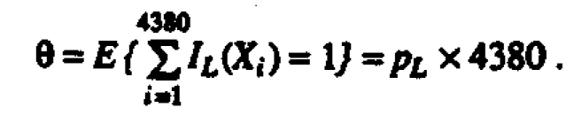
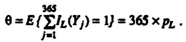
Suppose the random variable X represents a single hourly average reading for ambient ozone that is independently and identically distributed. (This simplifying assumption is not necessary for application of this approach but it is made here for X and below for Y for ease of exposition. Similar remarks apply to the assumptions of a normal distribution and a particular value of σ₂ stated below.) Denote by _PL =Prob {I_L(X) =1} the probability that X exceeds the limit L = 0.08 ppm. I_L(x) is the indicator function, which is one for x >L and zero otherwise. A year consists of approximately n = 365 x 12 = 4380 hours of observations (data are only taken from 9:01 am to 9:00 pm LST). The expected number of hours per year above the limit is then

The probability that a site is declared to be in compliance (d.i.c.) is

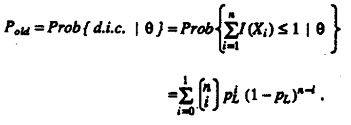
This probability P_old, plotted as a function of θ, is the operating characteristic curve for the old regulation (Figure 1). Note that if the old standard had been written in terms of an allowable limit of one for the expected number of exceedances above 0.08 ppm, the maximum type I error would be 1.00- 0.73 = 0.27. The old standard, however, is actually written in terms of the observed number of exceedances so type I and type II errors, strictly speaking, are undefined.

The condition of compliance stated in the new regulation is that the "expected number of days per calendar yes with daily maximum ozone" concentration exceeding 0.12 ppm must be less than or equal to 1."Let Y_j, represent the daily maximum hourly average (j = 1,. . . ,365). Suppose the random variables Y_j are independently and identically distributed. EPA proposed that the expected number of days (a parameter) be estimated by a three-year moving average of exceedances of 0.12 ppm. A site is in compliance when the moving average is less than or equal to 1. The expected number of days above the limit of L -0.12 ppm is then

The three-year specification of the new standard makes it hard to compare with the previous one-year standard. If, however, one computes the conditional probability that the number of exceedances in the present year is less than or equal to 0, 1, 2 and 3 and multiplies that by the probability that the number of exceedances was 3,2,1 and 0, respectively, for the previous two years, one then obtains a one-year operating characteristic function.

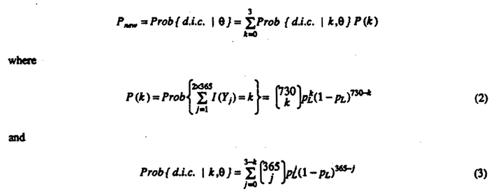
where k-0,1,2,3. A plot of the operating characteristic function for the new regulation, P_new versus θ, is presented in Figure 2 .

Figures 1 and 2 show the operating characteristic curves computed as a function of (1) the expected number of hours per year above 0.08 ppm for the old ambient ozone regulation and (2) the expected number of days per year with a maximum hourly observation above 0.12 ppm for the new ambient ozone regulation. We observe that the 95% de facto limit (the parameter value for which the site in a given year will be declared to be in compliance with 95% probability) is 0.36 hours per year exceeding 0.08 ppm for the old standard and 0.46 days per year exceeding 0.12 ppm for the new standard. If the expected number of hours of exceedances of 0.08 ppm is one (and therefore in compliance), the probability is approximately 26% of declaring a site to be not in compliance with the old standard. If the expected number of days exceeding 0.12 ppm is one (and therefore in compliance), the probability is approximately 37% of declaring a site to be not in compliance with the new standard. (We are unaware of any other legal context in which type I errors of this magnitude would be considered reasonable.) Note that the parameter value for which the site in a given year will be declared to be in compliance with 95% probability is 0.36 hours per year exceeding 0.08 ppm for the old standard and 0.46 days per year exceeding 0.12 ppm for the new standard.

Neither curve provides sharp discrimination between "good" and "bad" values of θ. Note that the old standard did not specify any parameter value above which non-compliance was defined. The new standard, however, specifies that one expected day is the limit thereby creating an inconsistency between what the regulation says and how it operates because of the large discrepancy between the stated limit and the operational limit.

The construction of Figures 1 and 2 only requires the assumption that the relevant observations are approximately identically and independently distributed (for the old standard, the relevant observations are chose for the hourly ambient ozone measurements for the new standard, they are the maximum hourly average measurements of the ambient ozone measurements each day). The construction does not require knowledge of the distribution of ambient ozone observations. If one has an estimate of this distributional form, however, a direct comparison of the new and old regulation is possible in terms of the concentration of ambient ozone (in units, say, of ppm.) To illustrate this point suppose the random variable X_i is independently and identically distributed according to a normal distribution with mean m and variance σ², that is, X_i ∼ N (µ, σ²). Then the probability of one observation being above the limit = L = 0.08 is

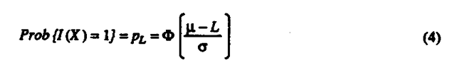
where Φi;( ) is the cumulative density function of the standard normal distribution. The probability that a site is declared to be in compliance can be computed as a function of μ by substituting _PL from (4) into (1).

For the new regulation let X_ij represent the one-hour average, (i = 1, . . . , 12;j = 1, . . . ,365), and Y_j = max {X_ij, . . . , X_i2,j}. If X_ij ∼ N (μ;, σ²), then Y_j ∼H(y) where

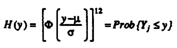
By substituting _PL in (2) and (3) with

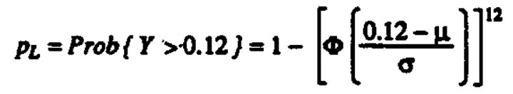
one obtains the operating characteristic function for the new standard.

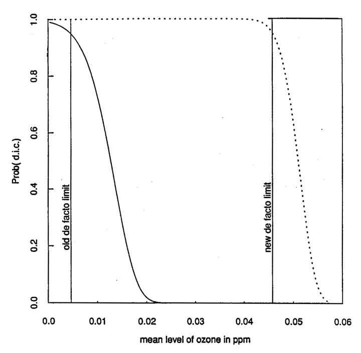
Figure 3. Operating characteristic curves for the old and new standards as a function of the mean value of ozone measured in parts per million when it is assumed that ozone measurements are normally and independently distributed with σ= 0.02 ppm

For a fixed value of the variance σ², one can compute the operating characteristic curves for the old and new regulations to provide a graphical comparison of the way these two regulations perform. Figure 3 shows these curves for the old and new ambient ozone regulations computed as a function of the mean hourly values when it is assumed that σ = 0.02 ppm. We observe that the 95% de facto limit is changed from 0.0046 ppm to 0.045 ppm. That is, it is approximately ten times higher in the new ozone regulation.

We have three observations to offer with regard to the old and new regulations for ambient ozone standards. First notwithstanding EPA's comment to the contrary, the new ozone regulation is not more statistical than the previous one; like all environmental regulations, both the new and old ozone regulations contain statistical parts, and, for that reason, both are statistical. Changing the specification from one in terms of a critical value to one in terms of a parameter does not make it more statistical. It actually introduced an inconsistency.

The old standard did not specify any parameter value as a limit but only an operational limit in terms at the parameter. This therefore constitutes the standard. The new standard, however, specifies not only an intent in terms of what the desired limit is but also an operational limit. The large difference between the interned limit and the operational limit constitute the inconsistency. This inconsistency is a potential and unnecessary source of conflict. Second, the new regulation is dependent on the ambient ozone level for the past two years as well as the present year, which means that a sudden rise in the ozone level might be detected more slowly. The new regulation is also more complicated. Third, it is unwise first to record and store every single hourly observation and then to use only the binary observation as to whether the daily maximum is above or below 0.12 ppm. This procedure wastes valuable scientific information. As a matter of public policy, it is unwise to use the data in a binary form when they are already measured on a continuous scale. The estimate of the 1/365 percentile is an unreliable statistic. It is for this reason that type I and type II errors are as high as they are. In fact, the natural variability of this statistic is of the same order of magnitude as the change in the limit which was so much in debate.

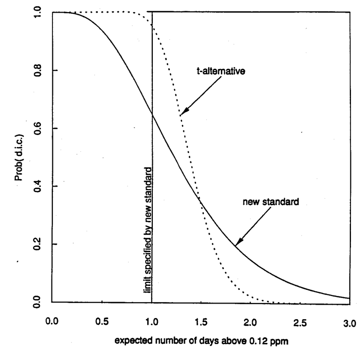
Figure 4. Operating characteristic curves for the new ozone standard and t-static alternative as a function of the expected number of exceedances per year.

If instead, for example one used a procedure based on the t-statistic for control of the proportion above the limit, as is commonplace in industrial quality control procedures (4), one would get the operating characteristic curve plotted in Figure 4 (see also appendix). For comparison, the curve for the new regulation is also plotted as a function of the expected number of exceedances per year. With the new ozone regulation, the probability can exceed 1/3 that a particular site will be declared out of compliance when it is actually in compliance. The operating characteristic curve for the t-test is steeper (and hence has more discriminating power) than that for the new standard. The modified procedure based on the t-test generally reduces the probability that sites that are actually in compliance will be declared to be out of compliance. In fact, it is constructed so that there is 5% chance of declaring that a site is out of compliance when it is actually in compliance in the sense that the expected exceedance number is one per year. Furthermore, when a violation has occurred, it is much more certain that it will be detected with the t-based procedure. In this respect the t-based procedure provides more protection to the public.

We do not conclude that procedures based on the t-test are best. We merely point out that there are alternatives to the procedures used in the old and new ozone standard. A basic principle is that information is lost when data are collected on a continuous scale and then reduced to a binary form. One of the advantages of procedures based on the t-test is that they do not waste information in this way.

The most important point to be made goes beyond the regulation of ambient ozone; it applies to regulation of all pollutants where there is a desire to limit exposure. With the aid of operating characteristic curves, informed judgements can be made when an environmental regulation is being developed. In particular, operating characteristic curves for alternative forms of a regulation can be constructed and compared before a final one is selected. Also, the robustness of a regulation to changes in assumptions, such as normality and statical independence of observations, can be investigated prior to the promulgation. Note that environmental lawmaking, as it concerns the design of environmental regulations, is similar to design of scientific experiments. In both contexts, data should be collected in such a way that clear answers will emerge to questions of interest, and careful forethought can ensure that this desired result is achieved.

Scientific Frameworks

The operating characteristic curve is only one component in a more comprehensive scientific framework that we would like to promote for the design of environmental regulations. The key elements in this process are:

• (a) Dose/risk curve
• (b) Risk/benefit analysis
• (c) Decision on maximum acceptable risk
• (4) Stochastic nature of the pollution process
• (e) Calibration of measuring instruments
• (f) Sampling plan
• (g) Decision function
• (h) Distribution theory
• (i) Operating characteristic function

Currently there may be some instances in which all of these elements are considered in some form when environmental regulations are designed. Because the particular purposes and techniques are not explicitly isolated and defined, however, the resulting regulations are not as clear nor as effective as they might otherwise be.

Often the first steps towards establishing an environmental regulation are (a) to estimate the relationship between the "dose" of a pollutant and some measure of health risk associated with it and (b) to carry out a formal or informal risk/benefit analysis. The problems associated with estimating dose / risk relationships and doing risk/benefit analyses are numerous and complex, and uncertainties can never be completely eliminated. As a next step a political decision is made - based on this uncertainties can never be completely eliminated. As a next step a political decision is made - based on this uncertain scientific economic groundwork - as to the maximum risk implies, through the dose/risk curve, the maximum allowable dose. The first three elements have received considerable attention when environmental regulations have been formulated, but the last six elements have not received the attention they deserve.

The maximum allowable dose defines the compliance set Θ₀ and the noncompliance set Θ₁, which is its complement. The pollution processcan be considered (d) as a stochastic process or statistical time-series Φ(θt). Fluctuations in the measurements X can usefully be thought of as arising from three sources: variation in the pollution level itself Φ, the bias b in the readings, and the measurement error ε. Thus X = Φ + b + ε. Often it is assumed that Φ = θ, a fixed constant and that variation arises only from the measurement error ε however, all three components Φ, b, and ε can vary. Ideally b = 0 and the variance of e is small.

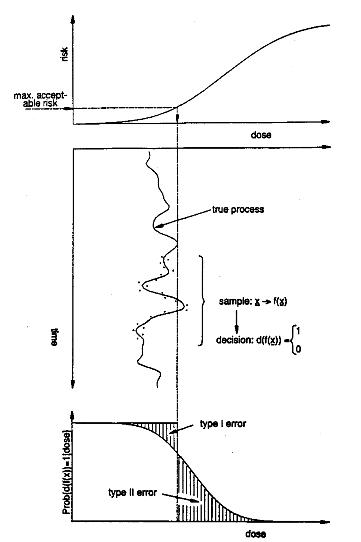
Figure 5. Elements of the environmental standard-setting process: Laboratory experiments and/or epidemiological studies are used to assess the dose/risk relationship. A maximum acceptable risk is determined through a political process balancing risk and economic factors. The maximum acceptable risk implies a limit for the "dose" which again implies a limit for the pollution process as a function of time. Compliance with the standard is operationally determined based on a discrete sample x taken from a particular site. The decision about whether a site is in compliance is reached through use of a statistic ƒ and a decision function d. Knowing the statistical nature of the pollution process, the sampling plan, and the functional form of the statistics and the decision function, one can compute the operating characteristic function. Projecting the operating characteristic function back on the dose/risk relationship, one can assess the probability of encountering various levels of undetected violation of the standard.

Measurements will only have scientific meaning if there is a detailed operational description of how the measurements are to be obtained and the measurement process is in a state of statistical control. A regulation must include a specification relating to how the instruments are to be calibrated (e). These descriptions must be an integral part of a regulation if it is going to be meaningful. The subject of measurement is deeper than is generally recognized, with important implications for environmental regulation (5, 6, 7). The pollution process and the observed process as a function of time are indicated in Figure 5.

Logically the next question is (f) how best to obtain a sample X = (X₁, X₂. . . ,X_n) from the pollution process. The answer to this question will be related to the form of the estimator ƒ(X) and (g) the decision rule

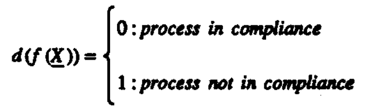
The sample, the estimator, and the decision function are indicated in Figure 5. Based on knowledge about the statistical distribution of the sample (h), one can compute (i) the operating characteristic function P = Prob {d (ƒ(X)) = 0 | θ} and plot the operating characteristic curve P versus θ. An operating characteristic function is drawn at the bottom of Figure 5. (In practice it would probably be desirable to construct more than one curve because, with different assumptions, different curves will result). Projected back on the dose/risk relationship (see Figure 5), this curve shows the probability of encountering various risks for different values of θ if the proposed environmental regulation is enacted. Suppose there is a reasonable probability that the pollutant levels occur in the range where the rate of change of the dose/risk relationship is appreciable then the steeper the dose/risk function, the steeper the operating characteristic curve needs to be if the regulation is to offer adequate protection. The promulgated regulation should be expressed in terms of an operational definition that involves measured quantities, not parameters. Figure 5 provides a convenient summary of our proposed framework for designing environmental regulations.

In environmental lawmaking, it is most prudent to consider a range of plausible assumptions. Operating characteristic curves will sometimes change with different geographical areas to a significant degree. Although this is an awkward fact when a legislative, administrative, or other body is trying to enact regulations at an international, national, or other level, it is better to face the problem as honestly as possible and deal with it rather than pretending that it does not exist.

Operating Characteristic Curve as a Goal, Not a Consequence

We suggest that operating characteristic curves be published whenever an environmental regulation is promulgated that involves a pollutant the level of which is to be controlled. When a regulation is being developed, operating characteristic curves for various alternative forms of the regulation should be examined. An operating characteristic curve with specified desirable properties should be viewed as a goal, not as something to compute after a regulation has been promulgated. (Nevertheless, we note in passing that it would be informative to compute operating characteristic curve for existing environmental regulations.)

In summary, the following procedure might be feasible. First based on scientific and economic studies of risks and benefits associated with exposure to a particular pollutant a political decision would be reached concerning the compliance set in the form of an interval of the type 0 ≤ θ ≤ θ₀ for a parameter of the distribution of the pollution process. Second, criteria for desirable sampling plans, estimators, and operating characteristic curves would be established. Third, attempts would be made to create a sampling plan and estimators that would meet these criteria. The costs associated with different sampling plans would be estimated. One possibility is that the desired properties of the operating characteristic curve might not be achievable at a reasonable cost. Some iteration and eventual compromise may be required among the stated criteria. Finally, the promulgated regulation would be expressed in terms of an operational definition that involves measured quantities, not parameters.

Injecting parameters into regulations, as was done in the new ozone standard, leads to unnecessary questions of interpretation and complications in enforcement. In fact, inconsistencies (such as that implied by Prob {ƒ(X) ≤ = c | θ₀} = 37% for the new ozone standard) can arise when conceptual differences between c and θ₀ and between ƒ(X) and θ are ignored. What is needed is a more refined conceptual model than that which underlies current environmental regulations, a model that makes these distinctions and acknowledges type I and type II errors.

Research Needs

Research that is used in designing environmental standards has focused on the first three elements of our framework (a), (b), and (c). If the last six elements do not receive relatively more attention than they currently receive, the precision obtained in estimating risk may well be lost by the lack of precision in estimating compliance. The above analysis, therefore, points to the need to have research resources more evenly spread among all the key elements (a), (b), . . . , (i). Furthermore, more research needs to be conducted that takes a global view of how all the elements function together. It would be beneficial to analyze many of the already promulgated standards using the framework outlined above and in particular to compute operating characteristic curves. Such research will sometimes require the development of new distribution theory because standards typically use rather complex decision rules. Moreover, most environmental data are serially correlated and consequently the shape of the operating characteristic function will be affected. At present little statistical theory is developed to cope with this problem. Preliminary studies we have me show that operating characteristic curves for binary sampling plans as used in the ozone standard seem to be seriously affected by serial correlation. Monte Carlo simulation might prove a viable alternative to distribution theory in evaluating the operating characteristic function for complex decision rules and serially correlated time series.

In our discussion above we only considered one pollutant and its regulation. The interaction among several pollutants and other environmental factors, however, might create higher risks than would be anticipated from separate studies on the individual pollutants themselves. Such Issues are only beginning to be addressed (8).

A related issue is the problem of what constitutes a rational attitude towards risk. It seems irrational to impose strict standards for one pollutant when other equally hazardous pollutants have much more relaxed standards. A harmonization among standards seems desirable. In order to address such issues it is necessary to develop methods for comparing convolutions of probability of occurrence, dose/risk relationships, and operating characteristic functions for several pollutants simultaneously. This will require an extension of the framework outlined above to multiple pollutants. However, that framework can be used as a first step in attacking these more comprehensive problems that are so important to protecting our environment.

Conclusion

One of the purposes of environmental law, which has been defined as the rules for planetary housekeeping (9), is to prevent harm to society. Assessment of risk is one of the key issues in environmental lawmaking and continued research is needed on how to measure risk and make decisions regarding risk; but risk assessment is not enough. If laws with good operating characteristics are not designed, the effort expended on risk assessment will simply be wasted. With limited resources, we need to develop methods for economically and rationally allocating resources to provide high levels of safety. Ideally a system of environmental management and control should be composed of individual laws that limit potential risk in a consistent manner. The ideas outlined in this article give partial answers to two connected questions: (i) how can we formulate an individual quantitative regulation so that it will be scientifically sound and (ii) how can we construct a rational system of environmental regulations?

If the framework outlined above is used properly in the course of developing environmental regulations, some of the important operating properties of different alternatives would be known. The public would know the probabilities of violations not being detected (type II errors); industries would know the probabilities of being accused incorrectly of violating standards (type I errors); and all parties would know the cost associated with various proposed environmental control schemes. We believe that the operating characteristic curve is a simple yet comprehensive device for presenting and comparing different alternative regulations because it brings into the open many relevant and sometimes subtle points. For many people it is unsettling to realize that type I and type II errors will be made, but it is unrealistic to develop regulations pretending that such errors do not occur. In fact, one of the central issues that should be faced in formulating effective and fair regulations is the estimation and balancing of the probabilities of such occurrences.

Appendix

The t-statistic procedure is based on the estimator 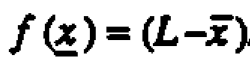is where L is the limit (0.12 ppm), the sample average, and s the sample standard deviation. The decision function is

The critical value c is found from the requirement that

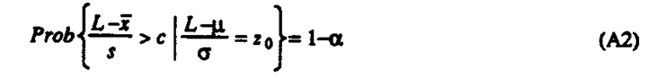
where z₀ = Φ^-1 (1-θ₀) and θ₀ is the fraction above the limit we at at want to accept (here 1/365).

The exact operating characteristic function is found by reference to a non-central t-distribution, but for all practical purposes the following approximation is sufficient

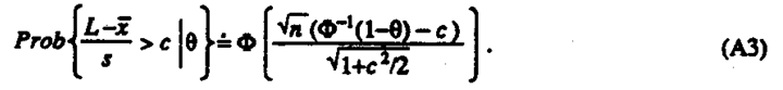
The operating characteristic function in Figure 4 is constructed using α = 0.05, θ ₀ = 01/365 and n = 3x 365. Substituting (A3) into (A2) yields

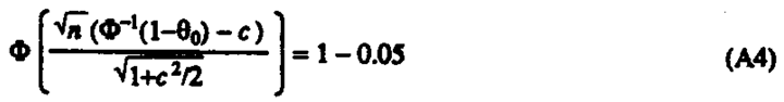
which solved for the critical value yields c = 2.6715. Refer for example to (4) for more details.

Literature Cited

1. National Primary and Secondary Ambient Air Quality Standards, Federal Register 36, 1971 pp 8186-187. (This final rulemaking document is referred to in this article as the old ambient ozone standard.)
2. National Primary and Secondary Ambient Air Quality Standards, Federal Register 44, 1979 pp 8202-8229. (This final rulemaking document is referred to in this article as the new ambient ozone standard.) The background material we summarize is contained In this comprehensive reference.
3. Javitz, H. J. J. Air Poll. Con. Assoc. 1980 30, pp 58-59.
4. Hald, A. "Statical Theory with Engineering Applications" Wiley, New York 1952 pp 303-311.
5. Hunter, J. S. Science 210, 1980 pp 869-874;
6. Hunter, J. S. In "Appendix D", Environmental Monitoring, Vol IV, National Academy of Sciences 1977;
7. Eisenhart, C. In "Precision Measurements and Calibration", National Bureau of Standards Special Publication 300 Vol. 1, 1969 pp 2I-47.
8. Porter, W. P. Hinsdill, R. Fairbrother, A. Olson, L. J. Jaeger, J. Yuill, T. Bisgaard, S. Hunter, W. G. K. Nolan, K. Science 1984, 224, pp 1014-1017.
9. Rogers, W. H. "Handbook of Environmental Law" West Publishing Company, 1977, St. Paul, MN.