A useful method for model-building II: Synthesizing response functions from individual components
williamghunter.net > Articles > A useful method for model-building II
by William G. Hunter and Andrzej P. Jaworski
February 1986
Practical Significance
There is a vast difference between quality control and quality improvement, passive statistical tools such as Shewhart control charts are useful for quality control, to determine whether the process under surveillance shows any signs of going out of its state of statistical control. On the other hand, more active tools are needed for quality and productivity improvement. In order to improve a process or a product, it is often helpful to use experimental designs in developing a mathematical equation or set of equations to relate the response(s) of interest to important process and environmental variables. Such models can aid in understanding how the relevant processes work so they can be modified in desirable ways. This report contains a practical suggestion that model-builders may find helpful. It involves synthesizing response functions of interest by starting with the simpler task of constructing models for component responses or subsets of them.
Key Words: Model-building, response surfaces, factorial design, component responses, synthesizing models.
Abstract
In model-building investigations the response of interest y is often a function of two or more components. The usual procedure in such situations is to use this function to compute the values of y for each run and then obtain the fitted equation 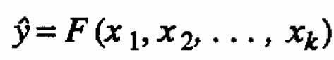 ?relating
  to relevant process variables. In this paper we suggest a different method that will sometimes be preferable: first fit equations to the component responses (either individually or in subsets) and then combine this these equations to obtain the desired function F. The proposed method is especially useful when the usual procedure fails to produce a satisfactory model. A chemical example illustrates how, by using this method, a second-order model can be obtained from a first-order design (a two-level factorial design).
1. Introduction
Frequently in model-building work the most important dependent variable is not measured directly but is calculated from other quantities. For example, (1) yield is sometimes computed by multiplying the recorded values of conversion and selectivity, and (2) profit is usually calculated from several measured quantities.
Using a simple chemical example for illustration, we show that useful models can sometimes be developed by fitting equations to more primitive measurements and then manipulating these equations to construct a model for the dependent variable (response) of interest. This method is in contrast to the standard procedure of first calculating the value of the response of interest for each experimental run and then fitting an equation to these values. By employing the method we propose, an investigator may be able to construct more flexible models that can provide better estimates of the responses and greater insight into the behavior of the system under study.
A model is a set of one or more equations that represents the behavior of a particular physical or biological system. Model-building is the process, typically iterative, by which investigators attempt to construct an adequate model. An essential part of this process is checking a candidate model against data to determine whether there is serious lack of fit Statistical procedures are most useful when they aid not only in detecting such lack of fit but also in pinpointing its possible source, so that research workers are helped in the next stage of creating a better model (Box and Hunter, 1962). Models can be discussed in terms of being either primarily empirical or mechanistic (see, for example, Box, Hunter, and Hunter (1978)), or a mixture of the two. This last class can be called empirical-mechanistic (see, for example, Phadke, Box, and Tiao (1977)).
After studying a specific empirical model-building problem in Section 2 to illustrate the basic idea of the present paper, we discuss the more general situation in Page 5 Section 3. In Section 4 we address some problems of inference, especially as it relates to computation of the variance of the estimated response. Concluding remarks are given in Section 5, and mathematical details are relegated to appendices.
2. Chemical example
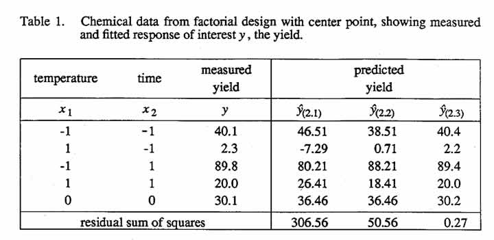
Consider the simple chemical reaction equation 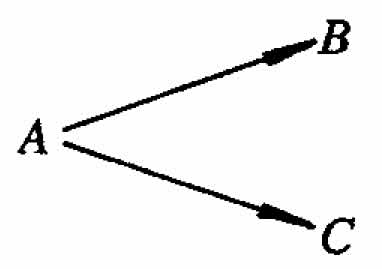 where A is the reactant, B is the product, and C is the by-product. Suppose a chemist is studying the effect of two controllable variables, temperature and time, on the yield of this reaction. Let x1 and x2 denote the coded values of these controllable variables. Suppose that a 22 factorial design with center point has been performed in random order, and the data shown in the first three columns of Table 1 are available.
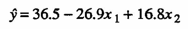
Using regression analysis to fit a standard first-order response surface model, one gets:
 (2.1)
(2.1)
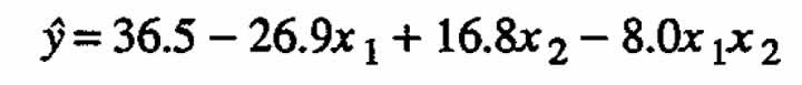
Suppose it is known that the standard deviation of y is less than 1%. The contour lines for this first-order equation for selected values of are shown in Figure 1(a) with the data points superimposed. It is evident from this figure as well as from the magnitude of the residual sum of squares (see column four in Table 1) that the first-order approximation is inadequate. If the model is assumed to include the interaction term, one obtains the following fitted equation:
 (2.2)
(2.2)
Contour lines for this model are shown in Figure 1(b). As would be expected, this response surface fits the data better than the first-order model however, there is still 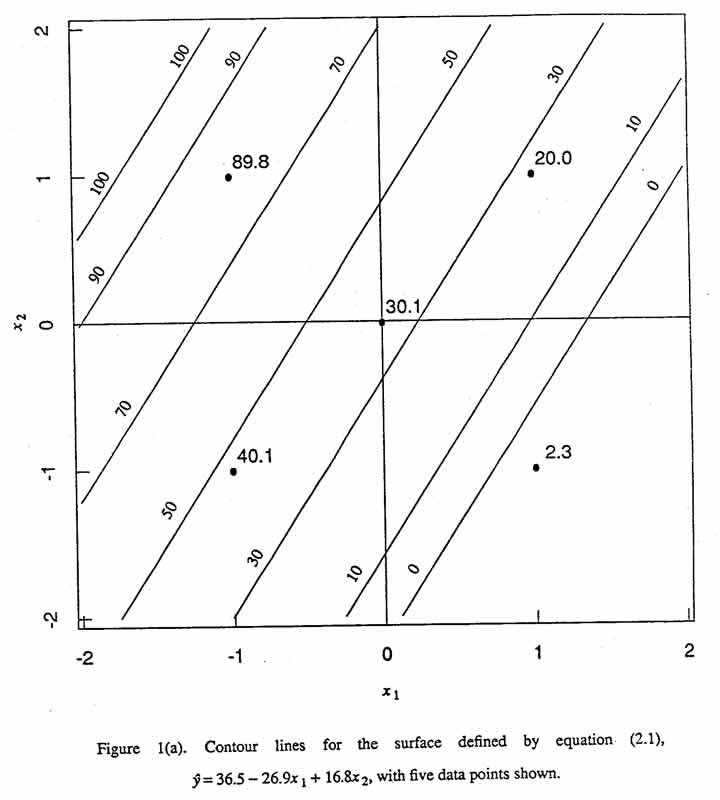
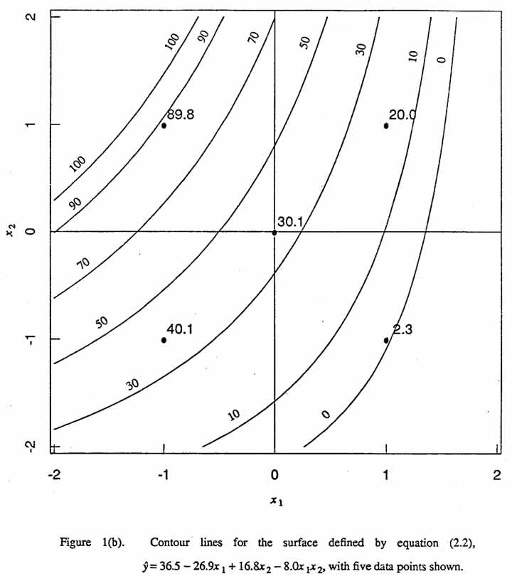 significant lack of fit caused mainly by the curvature of the response surface (see column five in Table 1)
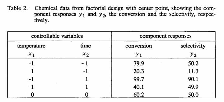
Suppose that the raw data for this model-building problem were those shown in Table 2 and that the yield y for each run was calculated as the product of the corresponding measured values of conversion y1 and selectivity y2, that is, y = y1y2 (To define these terms,  , where the square brackets denote the concentration of a chemical constituent and the subscript zero denotes the initial value. Conversion is, then, the fraction of the initial amount of reactant A that has reacted, and selectivity is the fraction of the amount of reactant A that has reacted that has been converted into product B.) The values of y1, y2 and y lie between zero and one, and they are often given as percentages. Fitting first-order response surface models to y1, and y2 separately gives
  Multiplying these two equations together and dividing by hundred to keep the yield results expressed in terms of percentages, we get:
 (2.3)
(2.3)
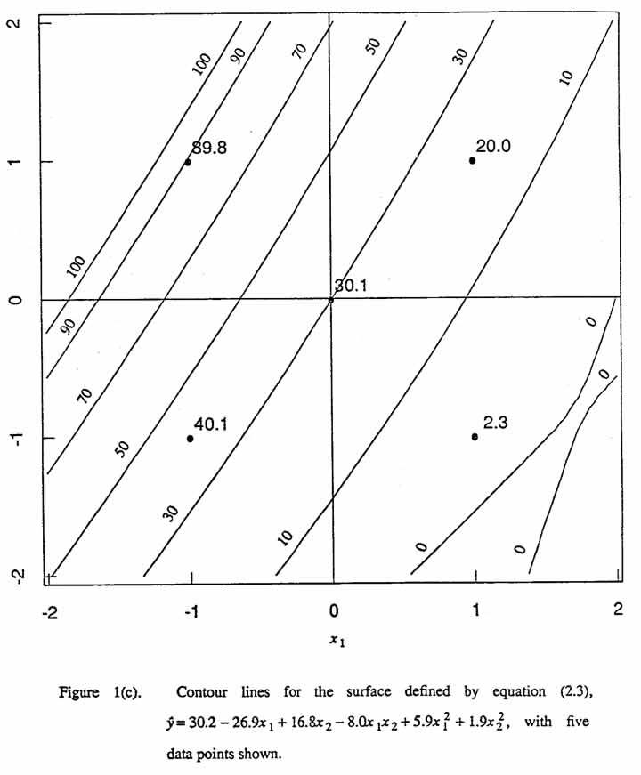
Contour lines for this model are shown in Figure 1(c). There is no detectable lack of fit for this second-order model. A canonical analysis for this equation is given in Appendix A (see, in particular, Equation (A.4)).
 (2.3)
(2.3)
Note that, by employing the above procedure, one is able to f?t a second-order model to data from a first-order design! Had the center point not been available, one could still have obtained a fitted second-order model.
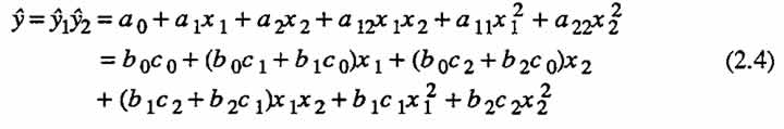
We now examine some interesting aspects of special second-order models that are derived in this way. Suppose that there are two first-order equations,  and the response of interest is the product of these two component responses. Then
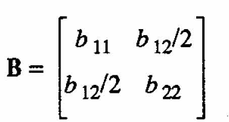
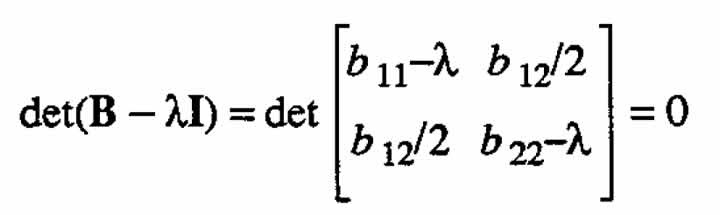
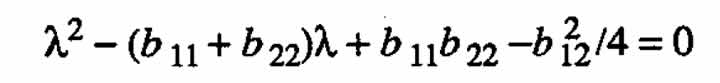
Can a model derived in the manner described above characterize all possible second order response surfaces? The answer is no. For the case when there are two variables, the eigenvalues ←mbda;1 and ←mbda;2 associated with the matrix of second-order coefficients
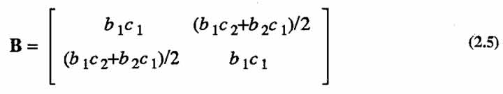
are constrained to be of different signs, or else one or both of these values must be zero. In other words, a second-order model constructed as described above does not have complete flexibility in that the two eigenvalues cannot be both strictly positive or strictly negative. (For proof, see Appendix B.) This means that the response surfaces exhibiting minimum or maximum cannot be represented by the synthesized model. (For details of canonical analysis see, for example, Myers (1971).)
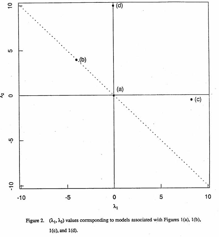
It is worthwhile to view this situation in the (←mbda;1, ←mbda;2) plane. Since the special second-order model (2.4) has eigenvalues of opposite sign or else at least one of the eigenvalues is zero, points cannot occur in the first or third quadrant of the (←mbda;1, ←mbda;2) plane. Four points are designated in Figure 2. Point (a), for (←mbda;1, ←mbda;2) = (0,0), corresponds to equation (2.1). Eigenvalues that are consistent with the general model form for a first-order equation with interaction fall along the dashed line. Point (b), for (←mbda;1, ←mbda;2) = (-4,4), corresponds to equation (2.2), an example of such a model. Point (c), for (←mbda;1, ←mbda;2) = (8.28, -0.48), corresponds to (2.3). The points (a), (b), and (c) in Figure 2, therefore, correspond to Figures 1(a), 1(b), 1(c), respectively. For more details on canonical analysis, see appendix A. To demonstrate flexibility of these special second order models, we show an additional contour map in Figure 1(d), which corresponds to point (d) in Figure 2.
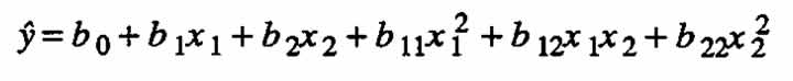
Let us examine each one of these four cases. Here we use the standard notation (see, for example, Myers (1971)) in which a general second-order model is written as
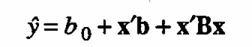
For the case of only two independent variables the above is usually written as
Case (a) ←mbda;1 = ←mbda;2 = 0.
This condition implies that B = 0 and that the prediction equation is first-order. Figure 1(a) shows the contour lines of a surface for such an equation, namely (2.1). Note that, for equal increments in , these parallel straight lines must be equidistant from one another.
Case (b) -←mbda;1 = ←mbda;2 = 4.
In general, ←mbda;1 = -←mbda;2 implies that >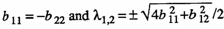 . For the special case b11 = b22 = 0, one obtains
  . Figure 1(b) shows contour Unes of a surface for this special case, corresponding to equation (2.2), for which -←mbda;1 = ←mbda;2 = 4.
Case (c) -←mbda;1 = 8.28, ←mbda;2 = -0.48.
Case (d) ←mbda;1 = 0,←mbda;2 = 10.
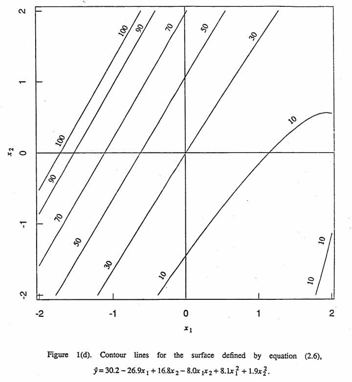
Because one eigenvalue is zero, it follows that  . Figure 1(d) shows contour lines of the surface for the following equation:
 (2.6)
(2.6)
which is equation (2.3) with b11 suitably altered so that ←mbda;1 = 0 and ←mbda;2 = 10.
3. The general method
In the chemical example above the response of interest y is related to two recorded quantities y 1 and y 2 by the simple function y = y1y2 , where there were two process variables x1 and x2. This example can be generalized in a number of ways. For instance, suppose the response of interest y is related to r observed component responses y1, y2,?,yr by the function y = f (y1, y2,?,yr) where there are k variables involved, x1, x2,?,xk. For this situation, the standard procedure for both empirical and mechanistic model-building is to calculate  for each run, u = 1, 2,?, n, and then to use these values to obtain a fitted model
Table 3. General set-up for building an adequate model F for the response of interest.Usual procedure: work first with rows, then the last column. Proposed method: work first with columns, then the last row.
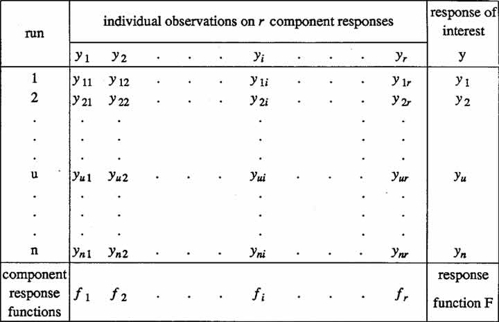
In terms of Table 3, one can visualize the standard procedure, in a sense, as getting to F in the lower right hand corner by first going across each row from left to right and then down the right column. In these terms, the main idea of this paper is that it will sometimes produce better results, in getting to F, to proceed first down each column and then from left to right across the bottom row: that is, (1) fit the data for each of the r responses y1, y2,?,yr individually, thereby obtaining r fitted component response functions 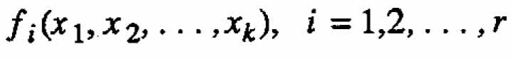 and then (2) obtain the final fitted response function F for y by appropriately combining the individual component functions. Equation (2.3) is an example of a function F, obtained this way.
In some situations, instead of fitting all r responses separately, it will be beneficial to combine some of them together in one or more subsets. Let us explain more specifically what we mean by such a subset with an example. Suppose there are five measured responses y1, y2,y3, y4, y5, and that the difference 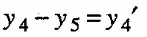 (say) is a meaningful and natural quantity for which the investigator chooses to develop a component model. This model for
  together with those for y1, y2, and y3 might them be used to synthesize a satisfactory model F. In this illustration, the pair of responses y 4 and y 5 constitutes an example of a reasonable subset to consider.
Whether one is using the standard procedure or the method described in this paper, it will be sometimes worthwhile - in addition to (or, in some cases that prove intractable, instead of) combining all the quantities y1, y2,?,yr together into a single response y - to study response functions for two or more component quantities. These response functions may be for the individual y1?s (i = 1,2,?, r) or some meaningful combinations of them. In fact, careful examination of such response relationships will usually lead to a better understanding of the overall system because one is thereby encouraged to reflect on the workings of some of its "component" parts. For this reason we recommend that such component response functions be studied, if possible in plotted form. In the chemical example considered in Section 2, for instance, it is beneficial to construct the first-order response surfaces for conversion and selectivity to learn how they relate to one another and to the response surface for yield.
We do not claim superiority in all model-building situations for analyzing the columns of the data matrix and then attempting to combine these results, rather than first combining the data for each row. In fact, see Box and Hunter (1962) for a striking example that illustrates how analyzing data in this way can sometimes unnecessarily complicate rather than clarify the situation. Note, however, that this example does not fit into the setup described in the present paper because the columns of the data matrix in that case are not component responses, equations for which are readily combined to obtain a model for the response of interest.
4. Inference
Let now consider the problem of estimating the precision of the fitted response. We will now treat a special example first and the general case second. In equation (2.3) the coefficients can be expressed as functions of the component coefficients. From equation (2.4) we have
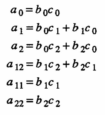
The coefficients a are bilinear forms of the component coefficients b and c. Hence, under the usual regression assumptions for the observed values y, one can apply the distribution theory of bilinear forms (see, for example, Seber (1977), pages 66-68) to calculate the variance-covariance matrix of the computed coefficients a. In principle one can then compute the variance of using standard linear model techniques (see, for example, Draper and Smith (1981), pages 83-84). Notice, however, that in this case a is no longer normally distributed, so the estimated variances will be only approximate.
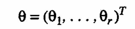
Let us now turn to the general case described in Section 3. The parameters of the synthesized response function F will not be expressible readily in terms of parameters of the component responses. Standard linear and nonlinear regression methods can be used to estimate the variance-covariance matrix of the parameters Θeta;i in the individual response functions fi. Joining all the component parameter vectors together, we obtain
with the block diagonal variance-covariance matrix
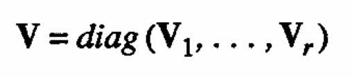
where Vi is the variance-covariance matrix for Θeta;i.
Under the usual assumptions the distribution of Θeta will be asymptotically normal, which will allow one to use known results specifying asymptotic normality of (see, for example, Serfling (1980)):
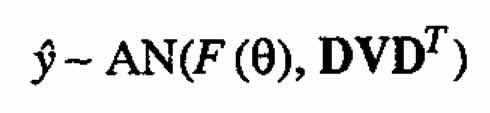
where
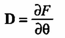
is the gradient of F with respect to Θeta;.
5. Conclusion
Model-building is typically an iterative process in which models are evolved, with inadequate ones being replaced by progressively improved versions see, for example, Hunter and Mezaki (1964), Blau and Neely (1975), and Ziegel and Gorman (1980). When the situation appears complex and an adequate model F is difficult to create following the usual route, progress may be possible by following the approach we describe because one can then deal with individual responses or reasonable subsets of them. Simpler component models would be expected to be adequate since experience indicates that, when responses are combined, complexities tend to increase rather than decrease. That is, it would be unusual for complexities in, say, a model for y1 and y2 to cancel one another so that the complexities in the model for the derived response  vanish or decrease. Exceptions can arise (see, for example, Box, Hunter, and Hunter (1978), page 533), but the more usual situation is illustrated by the chemical example in Section 2, in which the degree of complexity increases as one moves from the individual component models to that for the response of interest in that example the response surfaces for y1 and y2 are first-order, but that for y is second-order.
If the procedure described in this paper does not immediately give the best adequate model for the function F, it may give clues as to what forms might be useful to try. This method, which has been employed with success in the Institute for Industrial Chemistry in Warsaw, may prove to be most useful to model-builders when usual procedure fails to produce a parsimonious mathematical function that adequately fits the data. As always, any method for creating, fitting, evaluating, and using appropriate models has to be tailored to some extent for each problem. The appendices describe such a tailored analysis for the method discussed in this paper when it is used for the case of the chemical example introduced in Section 2.
Appendix a. Canonical analysis
We begin by considering the canonical analysis of the general second-order equation:
 (A.1)
(A.1)
The canonical form of this equation is  , where
  is the predicted value of response y calculated at the stationary point
  and ←mbda;1,?,←mbda;k are the eigenvalues of the matrix B.
For the two-variable case (k = 2), we have
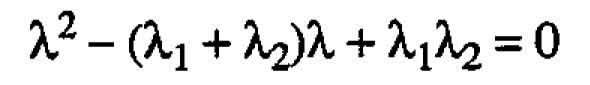
and the characteristic equation is
or
 (A.2)
(A.2)
Consider solutions of (A.2) that are consistent with the special second-order models of the form (2.4) derived by multiplication of two first-order models. As explained in Appendix B, the cigenvalues ←mbda;1) and ←mbda;2) must be of opposite sign or at least one eigenvalue must be zero. The following results show how the general second-order response surface model is constrained in three special cases.
Case 1. ←mbda;1 = ←mbda;2 = 0
Since (A.2) is equivalent to
or
it is clear, upon comparing these terms with those in (A.2), that 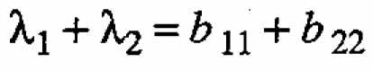 and
and 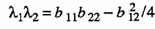 . Hence ←mbda;1 = ←mbda;2 = 0
Case2. ←mbda;1 = -←mbda;2
The solutions to (A.2) are
 (A.3)
(A.3)
Setting ←mbda;1 = -←mbda;2, we see that ?(b11 + b22) = b11 + b22 therefore that
b11 + b22= 0. Thus 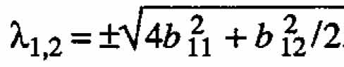 . If (A.l) is to represent a first-order model with interaction (, b11 = b22 = 0), then
 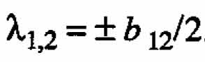 .
.
Case 3. ←mbda;1 ←mbda;2 = 0
In this case it follows from (A.3) that 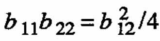 .
.
We now carry out a canonical analysis of (2.3). The matrix of the quadratic form is
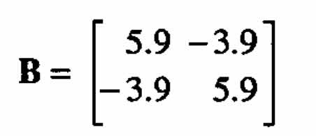
Hence its inverse is
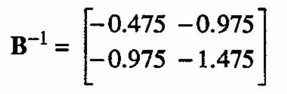
and the stationary point of this response surface is
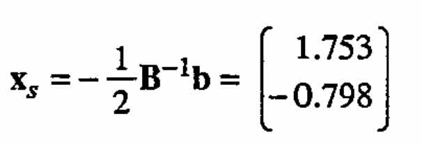
The estimated value of the response at the stationary point is  . (For special second-order models of the form (2.4)
  is always equal to zero.) After finding eigenvalues and eigenvectors of B we finally obtain the canonical form
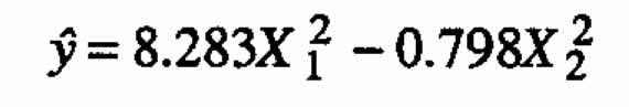
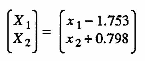
where the canonical variables are
Appendix B. Analysis of equation 2.4
This appendix contains an analysis of the special second-order model (2.4), which was obtained by multiplying together two first-order models. To simplify further discussion, let us initially consider the situation where both b1c1 and b1c1 are zero (2.4) is then no longer a full second-order model model. (Recall b11 = b1c1 and b22 = b2c2.) Four cases can be distinguished:
(1) b1 = 0 and b2 = 0. The model for y1c1 then reduces to a constant and model for y reduces to a first-order model.
(2) c1 =0 and c2 = 0. The same comment as above can be made with y2 substituted for y1.
(3) b1 =0 and b2 = 0.
(4) c1 =0 and b2 = 0. For both (3) and (4), the model for y becomes the first-order one with an added interaction term.
Let us now suppose that either b1c1 or b2c2, or both, are non-zero. Because of symmetry it is sufficient to consider only the single possibility, b2c2 &ne 0. We will examine the quadratic part of (2.4), specifically the matrix B given in (2.5), the determinant of which is equal to  .Hence det(B) ≤0 which implies that the quadratic form associated with B is indefinite. (This statement is true for any number of independent variables, because in any case B constitutes the first principal minor of the quadratic form. Hence the form can be neither positive nor negative definite (see, for example, Rao (1973)). Thus (2.4) cannot represent a response surface with an extremum, and consequently ←mbda;1 and ←mbda;2 cannot both be strictly positive or strictly negative.
References
Blau, G.E., and Neely, W.B. (1975), "Mathematical Model-Building with an Application to Determine the Distribution of Dursban Insecticide Added to a Simulated Ecosystem," Advances in Ecological Research, 9, 133-163.
Box, G.E.P., and Hunter, W.G. (1962), "A Useful Method of Model Building," Technometrics, 4, 301-318.
Box, G. E. P., Hunter, W. G., and Hunter, J. S. (1978), Statistics for Experimenters: An Introduction to Design, Data Analysis, and Model Building, New York: John Wiley Sons.
Draper, N., and Smith, H. (1981), Applied Regression Analysis (link to updated version 1998), New York: John Wiley & Sons. (2nded.)
Hunter, W. G. and Mezaki, R. (1964), "A Model-Building Technique for Chemical Engineering Kinetics," AI.Ch.E. Journal, 10, 315-322.
Myers, R.H. (1971), Response Surface Methodology, Boston: Allyn & Bacon, (reprinted by Edwards Bros., Ann Arbor, MI)
Phadke, M.S., Box, G.E.P., and Tiao, G.C. (1977), "Empirical-Mechanistic Modeling of Air Pollution", (in the proceedings of the 4th Symposium on Statistics and the Environment, March 3-5,1976)
Rao, C. R. (1973), Linear Statistical Inference and Its Applications, New York: John Wiley & Sons. (2nded.)
Seber, G.A. (1977), Linear Regression Analysis, New York: John Wiley.
Serfling, R. J. (1980), Approximation Theorems of Mathematical Statistics, New York: John Wiley & Sons.
Ziegel, E.R., and Gorman, J.W. (1980), "Kinetic Modelling with Multiresponse Data," Technometrics, 22, 139-151.
This research was supported in part by a grant from the Graduate School of the University of Wisconsin-Madison through the University-Industry Research Program and a grant from the National Science Foundation (DMS-8420968).
Computing was facilitated by access to the research computer at the Department of Statistics, Univerity of Wisconsin-Madison.