Articles and Reports by George E.P. Box

Statistics as a Catalyst to Learning by Scientific Method Part II-Discussion

Report No. 172

George Box
Copyright © June 1999, Used by Permission

Abstract

Part I of this article (Box and Liu, 1999) illustrates a number of concepts which together embody what I understand to be Response Surface Methodology (RSM). These ideas were originally introduced in a paper read to the Royal Statistical Society many years ago (Box and Wilson, 1951) and, as previously noted in Part I of this paper, have received considerable attention paper since that time. The present paper is about an aspect which I think needs to be further discussed. This concerns the implications raised when RSM is considered, as was originally intended as a statistical technique for the catalysis of iterative learning in the manner illustrated in part I of this paper. To introduce this topic I think I first need to explain how the paper referred to above came to be written.

Some History

While serving in the British army during the Second World War, I was, because of my knowledge of chemistry, transferred to a research station concerned with defense against chemical warfare. Biochemical results from animal experiments were extremely variable and since no professional statistical help was available, I was assigned the job of designing and analyzing many statistically planned experiments. J also helped to carry them out. My efforts over the next three years were necessarily based on self-study and most of the books and articles I was able to get were by R.A. Fisher and his followers. Later I studied statistics at University College London and in particular became familiar with Neyman-Pearson theory.

In 1948, my first job was at a major division of ICI in England. The people there were anxious to develop methods to improve the efficiencies of their many processes but my suggestion, that statistically designed experiments might prove helpful, was greeted with derision. The chemists and engineers said, "Oh, we've tried that and it didn't work." Enquiry showed that 4 for them, a statistical design had meant the advance planning of an all-encompassing "one shot" factorial experiment. This would test all combinations of the many experimental factors perceived to be important with each factor tested at a number of levels covering the whole of the ranges believed relevant.

A few of these very large factorial arrangements had, in fact, been begun but had quickly petered out. In the light of their knowledge of chemistry and engineering, after a few runs, the experimenters might say, "Now we see these early results, we realize that we should be using much higher pressures and temperatures. Also, the data suggest that some of the factors we first thought were important are not. We should be looking at a number of others not on the original list." The failures occurred because it was presumed the use of statistics meant that the whole investigation had to be planned when the experimenters knew least about the system. The result was that statistically planned experimentation received a very bad name.

It was clear that I had much to learn, so I joined a number of teams involved in process development and improvement.

I worked with them and particularly with a chemist K.B. Wilson who had considerable experience in that area. We watched what the experimenters did, and tried to find ways in to help them to do it better. It seemed that, most of the principles of design originally developed for agricultural experimentation would be of great value in industry, but the most industry experimentation differed from agricultural experimentation in two major respects. These I will call immediacy and sequentially.

What I mean by immediacy is that for most of our investigations the results were available, if not within hours, then certainly within days and in rare cases, even within minutes. This was true whether the investigation was conducted in a laboratory, a pilot plant or on the full scale. Furthermore, because the experimental runs were usually made in sequence, the information obtained from each run, or small group of runs, was known and could be acted upon quickly and used to plan the next set of runs. I concluded that the chief quarrel that our experimenters had with using "statistics" was that they thought it would mean giving up the enormous advantages offered by immediacy and sequentially. Quite rightly, they were not prepared to make these sacrifices. The need was to find ways of using statistics to catalyze a process of investigation that was not static, but dynamic.

Response surface methods were introduced as a first attempt to provide a suitable adaptation of statistical methods to meet these needs. It was a great surprise to us when Professor G.A. Barnard, then ICI's statistical consultant, suggested that our work be made the subject of a paper to be read before the Royal Statistical Society.

The Key Ideas of Response Surface Methods

It is necessary, I think, to reiterate the key ideas that were in the Box and Wilson (1951) paper. They are outlined below with references to the appropriate pages of the journal in which it was originally published. Points at which there were necessary injections of judgement and informed guesswork are indicated by italics.

1. Investigation is a sequential learning process. (p.2)
2. When there is little or no knowledge about the functional relationship connecting a response y and a group of factors x a truncated Taylor series Approximation ¹ (i.e. a polynomial in x of some degree d, usually 1 or 2) might produce a useful local approximation and the data themselves could suggest a suitable value for d. (p. 3)
3. When at the beginning of an investigation it is suspected that considerable improvement is possible, first order terms are likely to dominate. Factor screening and estimation can then be achieved by using two-level Plackett-Burman and fractional factorial designs followed by first order steepest ascent. (p. 10).
4. When, at a later stage first order terms appeared no longer dominant a higher degree polynomial, and in particular one of second degree, might be employed. (p.4)
5. When d is 2 or greater, factorial designs at d + 1 levels and their standard fractions obtained from group theory ² (Finney, 1945) are inappropriate and uneconomical for estimating the approximating polynomials. Instead, what were later called response surface designs, were used. These were classified, not by the number of levels used, but by the degree of the approximating polynomial they estimated. (p. 15)
6. For comparing bias properties of possible designs, the general alias matrix was derived. In particular, if a polynomial of degree d₁ was fitted when a polynomial of degree d₂ was needed, the alias matrix determined how the estimated coefficients would be biased. (p. 7)
7. By a process later called sequential assembly, a suitable design of higher order can be built up by adding a further block of runs to already existing runs from a design of lower order. For example, when the data indicates that this is necessary, a second order composite design may be obtained by adding axial and center points to a first order factorial or fractional.(p. 17) The general principle of "fold-over" is another example of sequential assembly which can be used when it is thought necessary to separate second order aliases from affects of first order. (p. 14, 16 and 35)
8. Real examples of experimentation with fractional two-level factorials used as first order screening designs followed by first order steepest ascent are given.(pp. 19, 20,21).
9. When earlier experimentation has exploited and greatly reduced dominant first order terms, it is likely that a near stationary region has been reached. Real examples showed how a second order approximating function might then be estimated and checked for model relevance and for lack of fit (later discussed more fully in Box and Wetz (1973) and Box and Draper (1987). (p.27)
10. When there are only two or three factors of major interest, contour plots and contour overlays can be of value in understanding the system. (p.3, 24 and 32)
11. More generally, canonical analysis of a second degree equation can indicate the existence of a maximum, minimum or, as in the helicopter example, a minimax. Also the type and direction of ridges can be determined. When, as is usual, there are costs and other responses that must be considered such ridges may be exploited to produce better than cheaper products and processes. (p. 24)
12. To check the reality of potentially interesting characteristics of the fitted surface, additional runs may be made at carefully chosen experimental conditions and, where appropriate, used in re-estimating the function. (p. 28)

Before proceeding further, I need to make a number of disclaimers.

1. RSM as described above represented a beginning. Later, these ideas were extensively developed by other researchers and other collaborators.
2. The detailed methodology of RSM is appropriate to a particular species of industrial problem. It is a certainly not intended as a cure-all. However, what has been made clear by my industrial experience, then and later, was that there should be more studies of statistics from the dynamic point of view. Unfortunately, with notable exceptions (see e.g. Daniel, 1961) the concept of statistics as a catalyst to iterative scientific learning has not received much attention by statistical researchers.
3. The illustrative investigation in Part 1 of this paper involves quite a number of experimental runs. Suppose, however, we were really in the business of making paper helicopters to achieve longer flight times and the original design represented the previously accepted state of the art. Then the increased flight time from 223 to 347 centiseconds achieved after only 21 runs using one fractional design and steepest ascent, could have put us far ahead of the competition. At this point, improvement efforts might, in practice, be halted temporarily. However, when competitors started to catch up, experimentation could begin in a manner corresponding to later parts of the example. Not surprisingly, as the product got better it would take more effort to improve it.
4. In the helicopter investigation only one response is considered (except in the early stages when dispersion is also analyzed). In most real examples there would be several responses.
5. The helicopter investigation is conducted almost entirely empirically. In practice, the result at each stage would be considered in the light of subject matter knowledge. This could greatly accelerate the learning process. Investigations must involve scientific feedback as well as empirical feedback.

¹ It was shown later (Box and Cox, 1964; Box and Tidwell, 1962) that the value of simple polynomial graduation functions can be increased considerably by allowing the possibility of transformation of y or of x.

² Three level designs of a different kind for fitting second degree equations were later developed by Box and Behnken (1960) that were specifically chosen to estimate the necessary coefficients in a second degree polynomial.

Statistics as a Catalyst to Learning

Francis Bacon (1561-1626) said "Knowledge Itself Is Power." The application to industry of this aphorism is that by learning more about the product, the process and the customer, we can do a better job. This is true whether we are making printed circuits, admitting patients to a hospital or teaching a class at a university.

Consider, as an example, an industrial investigation intended to provide a new drug which can cure a particular disease. There are two distinct aspects to this development:

• the long process of learning and discovery by which an effective and manufacturable chemical substance is developed;
• the process of testing it to ensure its effectiveness and safety for human use.

These two aspects parallel

• the tracking down of a criminal and the solution of a mystery by a detective;
• the trial of the criminal in a court of law.

Like the discovery and development of the new initially unidentified drug, the process by which a detective solves a mystery is necessarily a sequential procedure. It emphasizes hypothesis generation. It is based on intelligent guesswork inspired by clues which help decide what kind of data to seek at the next stage of the investigation. These procedures exactly parallel the sequential use of experimental design and analysis.

The trial of the accused, in a court of law is however, a much more formal process. It is a one-shot procedure, in which the court must make a decision taking account of very strict rules of already available and admissible evidence (past data). The "null hypothesis" of innocence must be discredited "beyond all reasonable doubt" for the defendant to be found guilty. By comparison, with this very formal trial process, the detective's methods for tracking down a criminal are informal and are continually concerned with the question: "given what I already known and suspect: How should I proceed? What are critical issues that need to be resolved? What new data should T try to get?" This process certainly cannot be put into any rigid mathematical framework. But in statistics, although research on "data analysis" led by John Tukey has gone part of the way to restore respectability to methods of exploratory enquiry, it still seems to be widely believed that expertise appropriate to aid the trial judge is also appropriate to advise the detective.

In particular the concept of hypothesis testing at accepted fixed significance levels are, so far as they can be justified at all, designed for terminal testing on past data of a believeable null hypothesis. They make little sense in the context of exploratory enquiry. We should not be afraid of discovering something. If know with only 50% probability that there is a crock of gold behind the next tree should I not go and look?

In the helicopter example, the informal use of normal probability plots ¹ is quite deliberate. We use the plots simply to indicate what might be worth trying. The idea that before proceeding further we need to discredit the already incredible null hypothesis (that the prototype design is the best possible) is clearly ridiculous².

It must be remembered that, except perhaps when dining with the Borgia's, the proof of the pudding is in the eating. When experimentation is sequential we need to think in terms of blitzkrieg rather than French warfare.

The analysis of variance in Table 4 is not intended to be used formally either. Its main purpose is to determine whether the fitted second degree equation is estimated sufficiently well to be worthy of further interpretation. In the example the occurrence of an F multiplier of 8.61 strongly suggests that it is. In the region covered by the design the F multiplier indicates whether the overall change in response predicted by the fitted equation is reasonably large compared with the error in estimating the response (Box and Wetz (1973), Box and Draper (1987)). For this purpose it is more appropriate than the more frequently used R².

Paradigm of Scientific Learning

The paradigm for scientific learning has been known at least since the time of Robert Grosseteste (1175 - 1253) who attributed it to Aristotle (384-322 BC). The iterative inductive-deductive process between model and data is not esoteric but is part of our every day experience. For example, suppose I park my car every morning in my own particular parking place. On a particular day after heave my place of work, I might go through a series of inductive-deductive problem solving cycles like this:

Model: Today is like every day.
Deduction: My car will be in my parking place.
Data: It isn't!
Induction: Someone must have taken it.

Model: My car has been stolen.
Deduction: My car will not be in the parking lot.
Data: No. It is over there!
Induction: Someone took it and brought it back.

Model: A thief took it and brought it back.
Deduction: My car will be broken into.
Data: No. It's unharmed and it's locked!
Induction: Someone who had a key took it.

Model: My wife used my car.
Deduction: She has probably left a note.
Data: Yes. Here it is!

Two equivalent representations of this process (which might be called the cycle and the saw-tooth) have been given respectively by Shewhart (1939) as modified by Deming (1982), and by Box and Youle (1955). They are shown in Figure 1. For example, the saw-tooth model indicates how data, which look somewhat different from what had previously been expected, can lead to the conception of a new or modified idea (tentative model) by a process of induction (I). By contrast, consideration of what the data would imply if the model were true is achieved by a process of deduction (D). The first implies a contrast indicated by a minus sign; the second involves a combination of data and model indicated by a plus sign³.

Studies of the human brain over the last few decades have confirmed that, in fact, separate parts of the brain are engaged in a conversation with each other to perform this inductive-deductive iteration. Thus although different people may follow different paths of reasoning, they can arrive at the same or equivalent conclusions.

¹Notice also that what is plotted are the averages of Peats runs. The variation in these averages thus includes "manufacturing" variation and is appropriate for conclusions about particular helicopters (see footnote #3 on pg. 4, part 1 of this article).

²However, if desired confidence cones about the directions of steepest ascent can be calculated (Box, 1954; Box and Draper, 1987). For the two steepest ascent paths calculated 95% confidence cones exclude, respectively, 97.9% and 94.7% of possible directing of advance.

³Some of the theoretical consequences of these ideas are discussed in Box (1980a. 1980b).

[Insert Figure 1 - not included in report as printed]

Notice that the acquiring of data may be achieved in many different ways, for example, by a visit to the library, by observing an operating system, or by running a suitable experiment. But to be most fruitful for all such activities subject matter knowledge must be available. For example, after the analysis of an initial experiment, a conversation between a scientific investigator and an inexperienced statistician could go something like this:

Investigator: "You know, looking at the effects of factors and x₂ and x₃ on the response y₁ together with how they seem to affect y₄₄ and y₅ suggests to me that what is going on physically is thus and so. I think, therefore, that in the next design we had better introduce the new factors x_i and x_j and drop factor x₁."

Statistician: "But at the beginning of this investigation I asked you to list all the important variables and you didn't mention x_i and x_j.

Investigator: "Oh yes, but I had not seen these results then."

While statisticians are accepted by scientists as necessary for the testing of a new drug, their value in helping to design the long series of experiments that lead to the discovery of the new drug is less likely to be recognized. For example, Lucas (1996) estimated that, of the 4000 or so members of ASA who were engaged in industry at that time, about 3000 were in the pharmaceutical industry - one suspects that a disproportionate number of these were concerned with rather than with the more rewarding and exciting process of discovery.

A Mathematical Paradigm

A purely mathematical education is focused on the one shot paradigm - "Provide me with a set of assumptions and, if some proposition logically follows, then I will provide a proof." Not surprisingly this mind-set can also produce a paradigm for hypothesis testing in mathematical statistics - "Provide me with the hypothesis to be tested, the alternative hypothesis and all the other assumptions you wish to make about the model, and I will provide an 'optimal' decision procedure." Similarly with experimental design - "Tell me what are the important variables, what is the exact experimental region of the interest in the factor space, what is the functional relationship between the experimental variables and the response, and I will provide you with an alphabetically optimal design. These are re quests to which most investigators would respond, "I don't know these things but I hope to find them out as I run my experiments."

By historical accident¹, experimental design was invented in an agricultural context. However the circumstances of agricultural experimentation are very unusual² and should certainly not be perceived as sanctifying methods in which all assumptions are fixed a priori and lead to a one-shot procedure. Iterative learning, of course, goes on in agricultural trials as elsewhere. The results from each year's trials are used in planning the next.

¹For example Fisher's earlier interest in aerodynamics could have resulted in a career in aircraft design perhaps producing a somewhat different emphasis in the design of experiments.

²Certain industrial life testing experiments are an exception.

Continuous Never Ending Improvement

We can better understand the critical importance of sequential investigation if we consider a central principle of modern quality technology - that of "Continuous Never Ending Improvement". This might at first be confused with mathematical optimization, but mathematical optimization takes place within a fixed model; by contrast, in continuous improvement, neither the functional form of the model, nor the identity of factors, nor even the nature of the responses is fixed. They all evolve as new knowledge comes to light. Furthermore, while optimization with a fixed model leads inevitably to the barrier posed by the law of diminishing returns, a developing model provides the possibility of continuous improvement and for expanding possibilities of return.

At the beginning of this century, Samuel Pierpont Langley - a distinguished scientist and a leading expert in aerodynamics with considerable financial support from the US government-built two airplanes designed largely from theoretical concepts. The planes were not operated by Langley himself and they never flew but fell off the end of the run way into the Potomac. By contrast the Wright brothers, after 3-years of iterative learning, first flying kites, then gliders, then powered aircraft, discovered not only how to design a working airplane but also how to fly it. (In the course of their investigations they also discovered that a fundamental formula for lift was wrong; they built their own wind tunnel and corrected it). Their airplane design, of course, was not optimal - any more than is that of the Boeing 777. The dimensionality of the factor space in air craft design, as in any other subject, is continually increasing.

It is obviously impossible to prove mathematical theorems about the process of scientific investigation itself, for it is necessarily incoherent; there is no way of predicting the different courses that independent experimenters exploring the same problem will follow. It is understandable, therefore, that statisticians inexperienced in experimental investigation will shy away from such activities and concentrate on development of mathematically respectable one-shot procedures. For such work it is not necessary to learn from, or cooperate with, anybody. To develop statistical decision theory, there was no need to consider the way in which decisions were actually made; nor, to develop the many mathematically optimal design criteria, was it ever necessary to be involved in designing an actual experiment.

Recently there has been considerable discussion of the malaise, which has affected statistical application. For example one of the sessions at the ASA annual meetings in 1997 was on the topic "The D. O. E. dilemma: How Can We Build on Past Failure to Ensure Future Success". I believe such discussion would be more fruitful if atlention was focussed on the Foot cause of such problems, namely the confusion between the mathematical and the scientific paradigm in determining much of what we do.

Success of the Investigation is the Objective

In the context of iterative learning, optimizations of separate designs and analyses will necessarily be sub-optimizations. It is the investigation itself, involving many designs and analyses that must be regarded as the unit and the success of the investigation as the objective. Although we cannot prove any mathematical theorems about the process of iterative investigation, we can apply ourselves to the study of the learning process itself. This should not be a matter for too much dismay. For example, after the discovery of the genetic code, geneticists of a biological turn of mind realized that, in addition to their previous knowledge, they must now acquire expertise in mathematical coding theory. We too ought to be able to make a transformation of this kind.

The Inductive Power of Factorial Designs

The floundering that we tend to do between the scientific and mathematical paradigms can lead to major misunderstandings. For example, I have often found myself defending the factorial design. "Surely," I am told, "with modem computers able to accomplish enormous tasks so quickly, you ought not to be content with outdated factorial designs." One can, of course, try to point out the design of a real experiment involves judgement and the wise balancing of many different issues with the help of the investigator. In addition, a different and very important point is usually missed. In favor of factorial designs is their enormous inductive power. Even if we grant that an "optimal" design might provide a useful answer to the question posed before we did the experiment, the experimental points from such a design are usually spread about in irregular patterns in factor space and of little use as a guide to what to do next.

One of the most fundamental means by which we learn is by making comparisons. We ask, "Are these things (roughly) the same or are they different?" A pre-school coloring book will show three umbrellas with the young reader invited to decide if they are the same or different. A factorial design is a superb "same or different machine." Consider, for example, a 2³ factorial design in factors A, B, and C represented as a cube in space in which a response y is measured at experimental conditions corresponding to each corner of the cube. By contrasting the results from the two ends of any edge of the cube, the experimenter can make a comparison in which only one factor is changed. Twelve such comparisons, corresponding to the 12 edges of the cube, can be made for each response. These basic comparisons can then be combined in various additional ways. In particular they can be used to answer the questions "On the average, are the results on the left hand side of the cube about the same as those on the right hand side (factor A main effect) or are they different? Are they on average the same on the front as on the back (factor B main effect) or are they different etc.?" Also, since an interaction comparison asks whether the differences produced by factor A are the same or different when factor B is changed, the possibility of interaction between the factors can be assessed by, similarly comparing the diagonals of the de sign. However as pointed out by Daniel, there are many natural phenomena which are not best explained in terms of main effects and interactions (or by polynomial functions). In particular a response may occur only when there is a "critical mix" of a number of experimental factors. For example, sexual reproduction can occur from a binary critical mix; to start an internal combustion engine requires a quaternary critical mix of gas, air, spark and pressure, and so forth. With a 2³ factorial design a tertiary mix is suggested as one explanation when one experimental point on the cube gives a response differing from all the others. A binary mix is suggested when two points on an edge are different from all the rest (see e.g. Hellstrand, 1989). Such possibilities can be suggested by a cube plot and by a normal plot of the original data. For this reason it seems best to decide first the space in which there is activity of some kind or other for a group of factors and to then decide what kind of activity is. Usually information will be come available simultaneously for not one, but for many different responses measured at each experimental point. This can provide an inspiring basis for the scientist or engineer using subject matter knowledge to figure out what might be happening and to help decide what to do next.

Projective Properties of Factorial Designs

Factorial designs are made even more attractive for purposes of screening and inductive learning by the discovery that certain two-level fractional factorials have remarkable projective properties (Box and Hunter, 1961). For example, a 2^8-4 fraction factorial orthogonal array containing sixteen runs can be used as a screen for up to three active factors out of eight suspects and supplies what was later called a (16,8, 3) screen (Box and Tyssedal, 1994, 1996). For this design every one of the 56 possible ways of choosing three columns from the eight factor columns produces a duplicated 2³ factorial design. The original 2^8-4 design can therefore be said to be of projectivity P =3. In addition to the fractional factorial arrangements for 4, 8, 16, 32,... runs a different kind of two-level orthogonal array is available for any number of runs that is a multiple of four (Placket and Burman, 1946). These arrangements will be called P.B. designs. They provide additional designs for 12, 20, 24, 28,... runs; some of these turn out to have remarkable screening properties. It was with some surprise that it was discovered first by computer search, that the 12 run P.B. design could screen up to 11 factors at projectivity P = 3 supplying a (12, 11,3) screen. (Box, et al, 1987, Box and Bisgaard, 1993). Furthermore Lin and Draper (1992) showed by further computer search that some but not all of the larger P.B. designs had similar properties. The conditions necessary for such designs to produce given projectivities were categorized and proved by Box and Tyssedal in the articles referenced above. Such screening designs are important because they can suggest which subset of the tested factors are, in one way or another, active. (See also Lin, 1993a,b, 1995).

Many designs have another interesting projective property that allows simple procedures to be used when the factor space is subject to one or more linear constraints. One such is the additive constraint which occurs when a set of factors measures the proportions of ingredients which must sum to unity. In particular, it was shown by Box and Hau (1998) that most of the operations of response surface methodology can be conducted by projecting standard designs and procedures onto the constrained space.

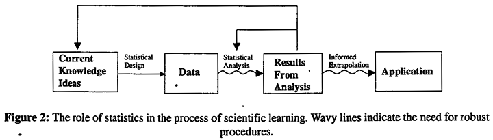
Robustness

If statistics is to be an essential catalyst to science, an important part of our job is to fashion techniques for continuous never-ending improvement that are suitable for use in the iterative learning cycles we have described. Such techniques rest on tentative assumptions (stated or unstated) and since all models are wrong, but some are useful, they must be robust to likely departures from assumption. As is indicated by the wavy lines in Figure 2 robustness concepts are important both for statistical analysis and also for the process of informed extrapolation required so that the results of an investigation can be put to practical use.

Robust Analysis

We first discuss the robustness of statistical analysis. It is sometimes supposed that if the assumptions are "nearly righ", then so will be a desired procedure and if they are "badly wrong", the derived procedure will not work. Both ideas are faulty because they take no account of robustness. As a specific example, consider the estimation of the standard deviation s with a control chart for individual items. Suppose an estimate is employed (see e.g. Duncan, 1974) based on the average moving range MR(bar) of successive observations. If it is assumed that the data are identically, normally and independently distributed then an unbiased estimate of a is provided by MR(bar)/l.128. But for data of this kind collected in sequence it is to be expected that successive deviations from the mean may be appreciably correlated. It can be shown (e.g. Box and Luceño, 1997) that even small serial correlations of this kind can seriously bias this estimate of σ.

In all such examples, the effect of a departure from as sumption depends on two factors: i) the magnitude of the deviation from assumption, ii) a robustness factor which measures how sensitive is the outcome to such a deviation. The concept is completely general, as is shown below, again using the correlation example for illustration.

Suppose that some outcome of interest (the estimate of s in the example but in general some characteristic of interest denoted by Y) is sensitive to an assumption about some characteristic (the zero value of the serial correlation coefficient for this example but in general some quantity defining the assumption denoted by Z). Now let a deviation z from assumption produce a change y in the outcome. Then approximately

and the effect y on the outcome is obtained by multiplying z, the discrepancy from assumption, by a robustness factor dy/dz, the rate of change of the outcome in relation to the change in assumption. Thus, as is well known, two different procedures even though derived from identical assumptions (such as a test to compare means by the analysis of variance, and a test to compare variances by Bartlett's test) can be affected very differently by the same departure from assumptions (the test to compare means is robust to most kinds of non-normality of the error distribution but the test to compare variances is not).

Such facts have led to the development of a plethora of robust methods. However practitioners must be cautious in the choice of such methods. In particular we should ask the question "robust to what?" For example, so-called "distribution free" tests recommended as substitutes for the t-test are just as disastrously affected by serial correlation as the t-test itself. When such sensitivity occurs, inclusion of the sensitive parameter in the formulation of the original model is often necessary to usually a robust procedure.

Robust Design

Almost never is an experimental result put to use in the circumstances in which it was obtained. Thus a result obtained from a laboratory study published in a Polish journal might find application in say, an industrial process in the United States. However, as was emphasized by Deming (1950, 1986), except in enumerative studies such a link with practice is hot made using statistics or formal probability, but by "a leap of faith" using technical judgement. Nevertheless the basis for that extrapolative judgment could be very strong or very weak depending on how the investigation was conducted; although no absolute guarantees are possible, by taking certain precautions in the experimental design process, we can make this job of informed extrapolation less perilous. Using statistics to help design a product that will operate well in the conditions of the real world is a concept that has a long history going back at least to the experiments conducted by Guinness's at the turn of the century. These experiments were run to find a variety of barley for brewing beer with properties that were insensitive to the many different soils, weather conditions and farming techniques found in different parts of Ireland.

Later Fisher (1935) pointed out that one of the virtues of factorial experiments was that, "(extraneous factors) maybe incorporated in experiments designed primarily to test other points with the real advantages, that if either general effects or interactions are detected, that will be so much knowledge gained at no expense to the other objects of the experiments and that, in any case, there will be no reason for rejecting the experimental results on the ground that the test was made in conditions differing in one or other of these respects from those in which it is proposed to apply the results."

We owe to Taguchi (1986) our present awareness of the importance of statistics in achieving robust processes and products in industry. Many such applications of robust design fall into one of two categories

1. minimization of the variation in system performance transmitted by its components
2. minimization of the affect on system performance of every day variation in environmental variables which occur in everyday use.

Overlooked solutions to both problems, in my view better than those later proposed by Taguchi, are due to Morrison (1937) and Michaels (1964). Morrison solved the first problem directly using the classical error transmission formula. He further made the critical observation that for any solution to be reliable, standard deviations of component errors must be reasonably well known (see also Box and Fung, 1986, 1993). Michaels showed how the solutions to the second problem are best dealt with as applications of split plot designs (see also Box and Jones, 1992 a and b).

It is clearly important that robustness concepts and response surface ideas should be considered together (see e.g. Vining and Myers, 1990; Kim and Lin, 1998). One illuminating approach to the environmental robustness problem can be understood by an extension of our earlier discussion. We assume in what follows that Taylor expansions that include derivatives up to the second order can provide adequate approximations.

As a specific example of environment robust design consider the formulation of a washing machine detergent (see Michaels, 1964). Suppose we have an initial "prototype" formulation (product design) for which, however, the effectiveness¹ Y is unduly sensitive to the temperature Z that is actually used in the domestic washing machine. To make it suitable for household use we need to modify the formulation so that the detergent's effectiveness is robust to a moderate departure z from the ideal washing temperature. If y is the change induced by z in the measure of effectiveness then as before approximately

¹Effectiveness of a detergent can be measured by applying a "standard soil" to a sample of white cloth and making a colorimetric determination of its whiteness after washing.

Now let dy/dz|p be the robustness factor for the initial prototype design and suppose we can find a design variable (say the proportion of compound X in the formula) which has a substantial interaction (measured by d²y/dzdx) with the temperature Z. Then the robustness factor can be changed in accordance with the equation

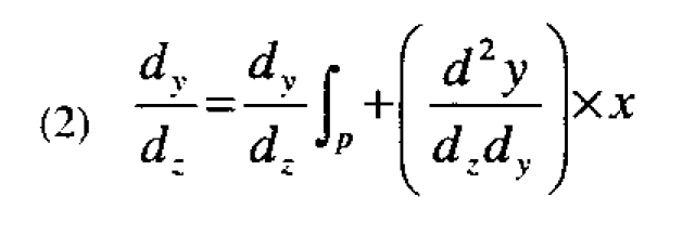
where x is the deviation of the design variable X from its value in the prototype formulation. Theoretically, therefore, the robustness factor can be reduced to zero and a formulation insensitive to temperature obtained by setting x=x* such that x* is the solution of the equation

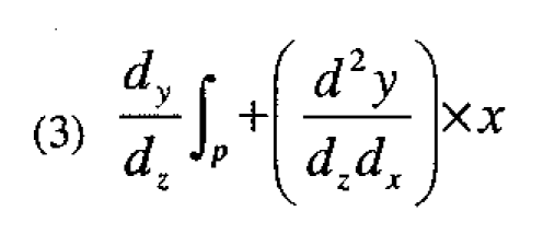
Now suppose we have a suitable experimental design centered at the prototype conditions x^• so that dy/dz|p can be estimated by the linear effect of the temperature (denoted below by c), and d²y/dzdx can be estimated by the interaction (denoted by C) of X with temperature. The value x* required for robustness can then be estimated from the equation

(4) -c=Cx*

More generally, suppose that in Equation 4, c now represents a vector of the linear effects of p environmental variables c = (c₁, c₂,. . . , c_p)' and C = {c_ij} represents a p × q matrix of interactions such that the element of its ith row and jth column is the interaction between the environmental variable Z and the design variable Xj. Then the solution of these equations x* = (x₁*, x₂*, . . . , x₄*), if such exists¹ , estimates the values of the design variables required for a robust design..

For illustration, suppose q = p = 2 and the environmental variables are Z₁, the temperature of the wash, and Z₂ its duration. Also suppose the design variables are the deviations from prototype levels of the amounts of two ingredients X₁ and X₂. Then the conditions x = (x₁ , x₂,...., x₀) which satisfy the robustness criterion are such that

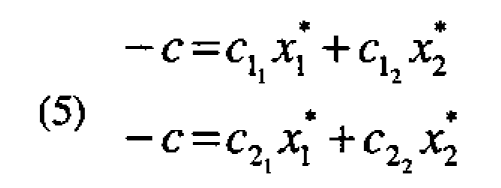
where it must be remembered that the coefficients c₁₁, c₁₂, etc. are all interactions of the environmental variables with the design variables. Thus, for example, c₁₁ is the interaction coefficient of Z₁ with X₁.

Notice that no account of the level of response (the effectiveness of the detergent) is taken by these equations. The robust formulation could give equally bad results at different levels of the environmental variables.

Now suppose that the environmental variables are at their fixed nominal values and that locally the response is adequately represented by a second degree equation in the design variables

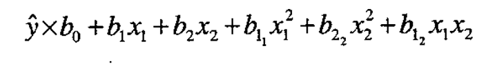
The coordinates 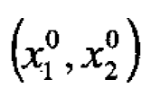of a maximum in the immediate region of interest will then satisfy the equations

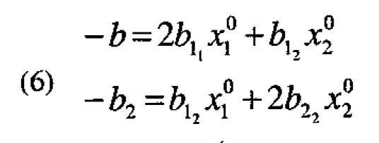
Note that these equations have no coefficients in common with the robustness equations (5).

Thus you could have an "optimal" solution that was highly non-robust and a robust solution that was far from optimal. In practice some kind of compromise is needed. This can be based on costs, the performance of competitive products and the like. One approach, which combines considerations of robustness and optimality and provides a locus of compromise between the two solutions, was given by Box and Jones 1992a, 1992b who showed which coefficients needed to be estimated to achieve various objectives, and provided appropriate experimental designs.

¹If there are more design variables than environmental variables (q>p) then an infinity of solutions may exist. If q = p and the matrix C is non-singular there will be a unique solution, and if q<p then no solution may exist. Also for the solution to be of any value, x* will need to be located in the immediate region where the approximations can be expected to hold and the coefficients in c and C will need to be estimated with reasonable precision. A discussion of the effects on the solution of errors in the coefficients of a linear equation is given for example in Box and Hunter, 1954.

Robust Design Using Split Plots

As Michaels (1964) pointed out, to achieve environmental robustness convenient and economical experimental designs are provided by split plot arrangements (Fisher, 1935, Yates, 1937) employing "main plots" and "subplots" within main plots. In industrial applications, situations requiring this kind of design are extremely common. In fact, the famous industrial statistician Cuthbert Daniel once said, perhaps with slight exaggerations that all industrial experiments are split plot experiments. The designs which Taguchi refers to as "inner" and "outer" arrays are usually split plot arrangements but have often not been correctly analyzed as such.

Depending on whether the design variables or the environmental variables are applied to the subplots, design main effects or environmental main effects will be estimated with the subplot error. In either case, however, all the de sign × environmental interactions would be estimated with the subplot error. Because it is frequently true that the subplot error is considerably smaller than the whole plot error the different kinds of split plot arrangements can have different theoretical efficiencies. These were given by Box and Jones (1992, b) who also who that strip-block designs can be even more efficient. They point out, however, that in practice the numbers of such operations and the difficulty and cost of carrying them out and are usually of most importance in deciding the way in which the experiment is conducted. In his experiment on different detergent formulations, Michaels applies the design variables (test products) to the subplots. When environmental conditions are not easily changed, this option can produce experimental arrangements which are much easier to carry out.

In practice of greatest importance is to discover which are the environmental factors whose effects need to be modified and to identify the design factors that can achieve this. The principle of parsimony is likely to apply to both kinds of factors. Fractional factorials and other orthogonal arrays of highest projectivity are thus particularly valuable to carry both the environmental and the design factors. Particularly when there are more design factors than environmental factors different choices or different combinations of design factors may be used to attain robustness. Relative estimation errors, economics and ease of: application can help decide the best optimum. Most important of all the nature of the interplay between designs and environmental factors revealed by the analysis should be studied by subject matter specialists. This can lead to an understanding of why the factors behave and interact in the way they do. Such study can produce new ideas and, perhaps, even better mean for robustification. Notice that these considerations require that we look at individual effects. Portmanteau criterion such as signal to noise ratios that mix up these effects are in my view unhelpful.

Teaching and Learning

How might the above discussion affect teaching? In the past teaching has often been regarded as a transference of facts from the mind of the teacher to that of the student. The mind, however, is not a good instrument for storage and retrieval of information. The computer can do it much better. What it cannot do is to solve unstructured problems. For this a great deal of practical experience is necessary including an understanding of the process of investigation. Thus a different approach to teaching is needed which is closer to that received by students and interns of medicine.

If it is to have a future therefore, I believe that statistics must be taught with much more emphasis on the iterative solution by students of unstructured problems, with the teacher adopting the role of mentor. Also, as well as its use for calculations and graphic display of results, greater emphasis should be placed on the use of the computer for search and retrieval. All the mind really needs to be taught is how and where to look. (see for example Box, 1997)

Fast Computation

There are many ways in which intensive computation, in conjunction with appropriate approximation, can help to catalyze learning. In particular, computer graphics can allow the investigator to look quickly at the data from many different viewpoints and to consider different tentative possibilities. Another application where intensive computation is essential to deductive learning is in the analysis of screening designs such as are mentioned above. For example, the 20 × 20 orthogonal array of Plackett and Burman is a (20, 19, 3) screen that can be used to screen up to 19 factors at projectivity 3 with only 20 runs. However, there are 969 possible 3 dimensional projections producing partially replicated 2³ designs in the chosen factors. With so many possibilities it is hardly to be expected that the factors responsible for the majority of response activity can be tied down in a single iteration. It has been shown (Box and Meyer, 1993) how a Bayesian approach may be adopted to compute the posterior probabilities of the various factors being active. Also Meyer et al (1996) show how ambiguities may be resolved by running a further subset of experiments which maximize the expected change in entropy. After these additional experiments have been run, the posterior probabilities can be recalculated and the process repeated if necessary. In this and other ways intensive computation can play its part in the acceleration of iterative learning.

Fix It or Understand It?

An often unstated issue which sometimes causes confusion is whether an experimental design is to be used to "fix the problem" and/or is part of an effort to "understand the problem." Thus, sometimes a faulty TV can be fixed at least temporarily by a carefully located and suitably modulated kick. At some point, however, the problem may need to be tackled by someone with subject matter knowledge who by a sequence of suitable tests, can learn what is wrong with the system and permanently put it right. The statistical practitioner can certainly feel that s/he has made some progress even if s/he is allowed only to demonstrate the power of a single highly fractionated design to fix a problem. This approach is demonstrated, for example, by the examples of Dr. Taguchi. S/he should not, however, feel satisfied with thus having dented resistance to the use of statistical methods. A modest success of this kind may sometimes provide the opportunity to point out with the statistical practitioner a valued member of the investigational team itself, statistics can contribute its full catalytic value to the learning process.

Statistics and the Quality Movement

I had earlier been pessimistic about the future of statistics. I was dismayed by the emphasis of statistics departments on matters that seemed of little interest to anyone but themselves and saddened, but not surprised, by the lessening support they were receiving from universities. It was particularly disturbing that this was happening at a time when the opportunities for the use of statistics and particularly experimental design in industrial investigations were growing at an unprecedented pace. Now, however, it is heartening to see how the quality movement is filling the gap. In particular, quality practitioners do not confine their activities to any narrow discipline but seem happy to learn and include whatever is required for the more efficient generation of knowledge in whatever sphere it is needed.

Conclusions

• Most industrial experimentation has a characteristic; here called immediacy, which means that results from an experiment are quickly known.
• In this circumstance investigations are conveniently conducted sequentially with results from previous experiments interacting with subject matter knowledge to motivate the next step.
• Such investigations use what may be called the scientific learning paradigm in which data drives an alternation between induction and deduction leading to change or modification of the model representing current knowledge.
• The iterative scientific paradigm is contrasted with the "one-shot" mathematical paradigm for the proofs of theorems.
• It is argued that because statistical training has unduly emphasized mathematics confusion between the two paradigms has occurred resulting in concentration on "one-shot" procedures within which mathematical theorems can be proven.
• Response surface methodology provides one means of iterative learning using factor screening, steepest ascent and canonical analysis of maxima and ridge systems.
• Factorial designs are defended as providing data which encourages inductive discovery. Projective properties of fractional factorials and other orthogonal arrays further assist this process.
• If statistical methods are to act as a catalyst to investigation, they must be robust to likely deviations from assumption. Necessary extrapolations of conclusions drawn from an experiment to application in the outside world can be strengthened by the use of robust design.
• Both the inductive and deductive investigational steps can be greatly strengthened by thhe present availability of massive resources for fast computation.
• The above conclusions have obvious implications to statistics learning and teaching.

References

• Box, G. E. P., Contribution to the Discussion on the Symposium on Interval Estimation, Journal of the Royal Statistical Society, Series B, 16, 211-212, 1954.
• Box, G. E. P., "Sampling and Bayes" Inference in Scientific Modelling and Robustness", Journal of the Royal Statistical Society, Series A, 143, 383-404, discussion 404-430, 1980a.
• Box, G. E. P., "Sampling Inference, Bayes' Inference and Robustness in the advancement of Learning", Bayesian Statistics, Bernardo, J. M., DeGroot, M. H., Lindley, D. V. and Smith, A. F. M. (eds.), Valencia, Spain: University Press, 366-381, 1980b.
• Box, G. E. P., "Statistics and Quality Improvement", Journal of the Royal Statistical Society, Series A, 157(2), 209-229, 1994.
• Box, G. E. P., "Scientific Method: The Generation of Knowledge and Quality", Quality Progress, 47-50, January 1997.
• Box, G. E. R and Benhken, D. W. "Some new three level designs for the study of quantitative variables", Technometrics, 2,455-475, 1960.
• Box. G. E. R and Bisgaard, Søren, "What Can You Find Out From 12 Experimental Runs?," Quality Engineering, Vol.5, No.4, 663-668,1993.
• Lucas, James M., The 1996 W.J. Youden Address: System Change and improvement: Guidelines for Action When the System Resists, ASA Proceedings, 1996.
• Meyer, R. Daniel, David M. Steinberg and G. E. P. Box, "Follow-up Designs to Resolve Confounding in Fractional Factorials," Technometrics, 38(4) 330-313, 1996.
• Michaels, S. E, "The usefulness of Experimental Designs (with discussion)," Applied Statistics, 13, 221-235, 1964.
• Morrison, S. J., "The Study of Variability in Engineering Design," Applied Statistics, 6, 133-138, 1957.
• Myers, Raymond H. and Montgomery, Douglas C., Response Surface Methodology, Process and Product Optimization Using Designed Experiments, New York, Wiley, 1995.
• Plackett, R. L. and Burman J. P., "The design of optimum multifactorial experiments," Biometrika, 33,305-325 and 328-332. 1946.
• Shewart, Walter, Statistical Method: From the Viewpoint of Quality Control, Lancaster Press, 1939.
• Taguchi, G., Introduction to Quality Engineering: Designing Quality into Products and Processes. White Plains, N. Y., Kraus International Publications, 1986.
• Yates, F., "The design and analysis of factorial experiments," Bulletin 35. Imperial Bureau of Soil Science. Harpenden Hens, England, Hafner (McMillan), 1937.