Articles and Reports by George E.P. Box
williamghunter.net > George Box Articles > Quality Improvement: the New Industrial Revolution
Quality Improvement: the New Industrial Revolution
Report No.74 in Quality and Productivity
George Box.
Copyright © October 1991, Used by Permission
Abstract
Beginning from Bacon's famous aphorism that "Knowledge Itself is Power", the underlying philosophy of modern quality improvement is seen as the mobilization of presently available sources of knowledge and knowledge gathering. These resources, often untapped include the following: (i) that the whole workforce possesses useful knowledge and creativity; (ii) that every system by its operation produces information on how it can be improved; (iii) that simple procedures can be learned for better monitoring and adjustment of processes; (iv) that elementary principles of experimental design can increase the efficiency many times over of experimentation for process improvement, development, and research.
Keywords: Quality improvement, process control, process monitoring, experimental design, robustness
The quality revolution which has transformed industry in Japan and is rapidly doing so elsewhere is concerned incidentally with quality but more fundamentally with the efficient acquisition of knowledge. Sir Francis Bacon made the profound observation that "Knowledge itself is Power". To the extent that we have more knowledge about our product, our process, our customer, and every part of our operation, we can use that knowledge certainly to produce better quality; but also to increase productivity, lower cost, increase through put and to do whatever we want to do.
Knowledge about our world is, and always must be, partial knowledge. Sir Ronald Fisher showed us how that partial knowledge can be most rapidly increased by the use of the efficient methods of statiscal analysis and experimental design which he devised. Partial knowledge about some characteristic, y, of a system is often expressed by the statistician in the form
where xk defines the levels of variables, or states of nature, "known" to effect y, and e is error or noise. A more detailed form of (1) is
where xu defines is the level of all the unknown variables which effect y. The F statistics, t statistics which Fisher devised or developed are all examples of what engineers call signal to noise ratios and are particular measures of what is known in relation to what is unknown. Increased knowledge about system is achieved by transfer of elements of xu, from the "e bracket" to the "ƒ bracket" as is illustrated in equation
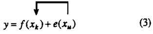
For example, the use of a quality control chart, a regression analysis, or an experimental design are all ways to achieve this end.
With this model in mind, die issue then is how to produce new knowledge efficiently using only those assets presently available to us-without new staff and without new machinery.
We have four things going for us:
- every operating system-manufacturing, billing, dispatching and so forth-produces information that can be used to improve it;
- every person has a creative brain as well as a pair of hands;
- process control techniques can lock in improvements and help to minimize variation about target values;
- statistical experimental design can reduce many times over the cost and effort of experimentation and in particular experimentation with many variables is essential to produce trouble-free products and processes.
Every Operating System Produces Information That Can Tell Us How To Improve It
Perhaps the most important "Law of Nature" is what, in the United States, is called Murphy's Law - "If something can go wrong with a system it will go wrong". But what do we mean by a system? The important example that immediately comes to mind is an industrial manufacturing process. But even in industry many systems are not concerned with manufacture but with invoicing, dispatching, billing, etc. It is important to remember that it is just as essential to get the bugs out of those systems as out of the process of manufacturing itself. But the kind of a system I'm talking about might have nothing to do with manufacturing. It might be baggage handling in an airline, student registration in a college or health care delivery in a hospital. If one listens to Murphy, all these systems can be improved.
Most of us think of Murphy as a great nuisance, but that's only if we don't listen to him. When I got on the airplane to come to this meeting, and I carried my speech in my hand rather than checking it with my luggage, I was being respectful to Murphy. If we listen to Murphy then, when something goes wrong, we don't blame anybody, we just make sure that that particular bad thing cannot happen again.
Three potent techniques to make Murphy work for us are: .
- corrective feedback-modifying the system so that a particular fault that has turned up can never happen again,
- preemptive feedforward-anticipating problems before they happen and devising foolproof systems which avoid them,
- simplification-rendering cach system and sub-system as straightforward as possible; see for example Fuller (1986).
Concerning simplification, in the past, systems have tended to become steadily more complicated. One reason is that "water runs downhill" and that complicated systems favor the bureaucracy. In many organizations over the years the proportion of time taken up by purely administrative matters required by the bureaucracy, has steadily increased. This has often prevented people from getting on with their real jobs. This problem appears equally in industry and in government, as well as other service organizations such as universities. Because an increase in the activity of a bureaucracy benefits its members but not necessarily the organization it serves, safeguards are needed to control it.
One such safeguard is a Consequential Impact Statement that the bureaucrat must complete before any new rule, procedure, form, or questionnaire can be approved. Some of the questions should be:
- How much time will this take?
- Using an average salary rate multiplied by the number of people involved, what is its nominal cost?
- Because the people involved are fully occupied now, what are the things that they will not now be required to do?
- What is the cost of not doing these things?
- Taking all of the preceding into account, is this substitution of activities wise?
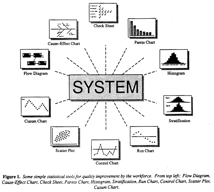
Not all information generated by a system and leading to improvement is about specific faults.More generally an operating system can be likened to a radio transmitter which is transmitting information on how the system can be improved. But just as we need radio and television receivers to decode the transmission, so we need simple tools to tap into the information coming from a process. One such set of simple statistical tools that almost everyone in the workforce can be trained to use has been described and demonstrated by the late Kaoru Ishakawa (1976) these with a few additions are indicated in Figure 1.
Every Person has a Creative Brain as Well as Pair of Hands
So far I have said that every process can provide me information on how it can be improved. But in the past this information was mostly ignored. It was remote from management who were in any case to "busy" to look at it. It was not realized that the work-people closest to the system could be trained and empowered to put it to use.
Creativity is the unique quality that separates mankind from the rest of the animal kingdom-and every human being possesses it. Just as "fish gotta swim and birds gotta fly", so an opportunity to use creativity is a vital riced for all humanity. The distribution in the work force of the ability to solve problems might look something like Figure 2a while the distribution of the problem solving ability required to solve the problems that routinely reduce the efficiency of factories, hospitals, bus companies and so forth might look something like Figure 2b.
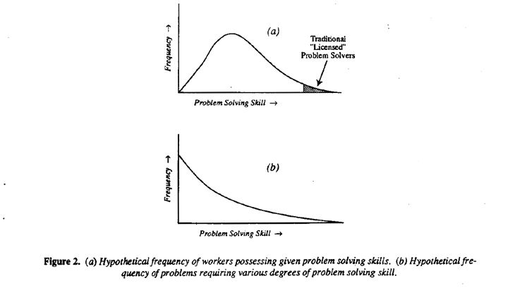
In the past, only those possessing highly trained scientific or managerial talent, would have been regarded as "licensed" problem solvers. Inevitably this small group could only tackle a small proportion of the problems that beset the organization and would often be too remote from the system to appreciate them. But ordinary people can understand the necessary ideas and use the elementary tools required for problem solving. They enjoy working in a team to solve the myriad of simple but expensive problems that beset every system. An organization that does not use this talent throws away a large proportion of its creative potential.
The bringing together of the two ideas:
- that every operating system provides information on how to improve it and
- that every human being has the ability to solve problems provides huge potential
- resource for improvement.
This is even more the case because, as Dr.'s Deming and Juran have both pointed out, it has been estimated that at least 85% of all problems concern the system (previously a preserve of management) and not the operation of the process by the work force Therefore, however careful the work force is, at least 85% of all the problems were not ordinarily within their power to correct. However, as soon as quality improvement teams are formed with management leadership which are empowered to find and correct faults and where necessary to redesign the system, this limitation no longer holds. The quality teams become, in effect, part of management.
This possibility is so obvious that one wonders why it has not more often been put into effect. Some reasons are given by W. Edwards Deming in his classic book Out of the Crisis. In particular bringing about the necessary changes requires:
- A radically different management philosophy.
- An appropriate organization to put this philosophy into effect.
By far the most difficult change that is needed is a change of management philosophy. The old fashioned idea of good managers is that they know all the answers, can solve every problem alone, and can give appropriate orders to subordinates to carry out their plans. This is a role that is seldom possible to sustain with comfort or without hypocrisy. Good modern managers are like coaches who lead and encourage their teams in never-ending quality improvement. While some managers are enthusiastic about their new role, others find such a change threatening and associate it with loss of power. It is hard to have been selected to be a good "sergeant major" - and then to find what was really required was a good coach.
Process Control Techniques
Good quality usually requires that we reproduce the same thing consistently. If, for example, we are manufacturing a particular part for an automobile, we would like each item to be as nearly identical as possible. It would be nice if this could be achieved, once and for all, by carefully adjusting the machine and letting it run. Unfortunately this would rarely, if ever, result in the production of uniform product. In practice extraordinary precautions are needed to ensure near uniformity. Again, consider some routine task in a hospital, such as the taking of blood pressure: having found the best way to do this, we would like it to be done that way consistently, but experience shows that very careful planning is needed to ensure that this happens.
Process control is a continuous attempt to undo the effects of the second law of thermodynamics which says, that all processes if left to themselves, the entropy (the amount of disorder in the system) will either stay constant or increase.
The truth is that the idea of stationary - of a stable world in which, without our intervention, things stay put over time, is a purely conceptual one. The concept of stationary is only useful as a back-ground against which the real non-stationary world can be judged. For example, the manufacture of parts is an operation involving machines and people. But the pans of a machine are not fixed entities. They are wearing out, changing their dimensions, and losing their adjustment the behavior of the people who run the machines is not fixed either. A single operator forgets things over time and alters what he does. When a number of operators are involved, the opportunities for involuntary changes because of failures to communicate are further multiplied. Thus, if left to itself any process will drift away from its initial state. So the first thing we must understand is that stationarity and hence, uniformity of everything depending on it, is an unnatural state that requires a great deal of effort to achieve.
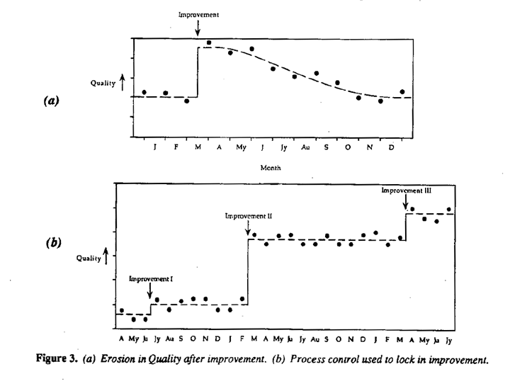
Now this paper is about Quality lmprovement; about changing things for the better, but Quality Control is about keeping things constant. These aims, however, are not inconsistent. The way that they fit together has been described for example by Juran (1988) and by Imai (1986). By using the simple tools referred to earlier, quality teams will almost inevitably find better ways to do things. Unfortunately, experience shows that if nothing is done to prevent it, the improved quality, so hardly won, may gradually disappear.
Over a period of time, carefully adjusted machines become untuned and people forget, miscommunicate and become less careful in their work. In the natural course of events, therefore, quality will erode in the way illustrated in Figure 3a. What we must do is to lock in improvements, so that at each stage the new higher level of quality is maintained, as is Figure 3b.
If you ask a statistical quality control practitioner and a control engineer what they would do about this, you are likely to receive very different answers. On the one hand, the quality control practitioner will most likely talk about the uses of Shewhart charts and possibly some more recent innovations such as Cusum charts and EWMA charts for process monitoring. On the other hand, the control engineer will likely talk about process regulation - feedback and feedforward control, proportional-integral controllers and so forth.
Both the quality control practitioner's concepts and those of the control engineer are highly important and both have long and distinguished records of practical achievement. My purpose here is to underline the nature of the different contexts, objectives, and assumptions of their operation and to show how some of the ideas of the control engineer can be readily adapted by the statistical quality practitioner to deal with certain problems of process adjustment with which he is often faced.
Process Monitoring and Process Regulation: Context, Objectives, and Assumptions
Process Monitoring,whether by the use of Shewhart charts (or for example by Cusum or Exponentially Weighted Moving Avenge charts), is conducted in the context that it is feasible to bring the process to a basic state of statistical control by removing causes of variation. A state of statistical control implies stable random variation about the target value produced by a wide variety of "common causes" whose identity is currently unknown. In a Shewhart chart this stable random variation about the target value provides a "reference distribution" against which apparent deviations from target can be judged in particular by the provision of "three sigma" and "two sigma" limit lines. It is only when a improbable deviation from this postulated state of control occurs that a search for an assignable or "special" cause will be undertaken. This makes sense in the implied context that the "in control" state applies most of the time and that we must be careful to avoid spending time and money on "fixing the system when it ain't broke". The objectives of process monitoring are thus (a) to continually confirm that the established common cause system remains in operation and (b) to look for deviations unlikely to be due to chance that can lead to the tracking down and elimination of assignable causes of trouble.
Now, while we should always make a dedicated endeavor to bring a process into a state of control by fixing causes of variation such as differences in raw materials, differences in operators and so forth, some situations occur, which cannot be dealt with in this way; in spite of our best efforts, there remains a tendency for the process to wander off target. This may be due to naturally occurring phenomena such as variations in ambient temperature, humidity and feedstock quality or they may occur from causes which currently are unknown. In such circumstances, some system of regulation may be necessary.
Process Regulation by feedback control* is conducted in the context that there exists some additional variable that can be used to compensate for deviations in the quality characteristic and so to continually adjust the process to be as close as possible to target. In this article "as close as possible" will mean with smallest mean square error (or essentially with the mean on target and with smallest standard deviation about the mean). What I am talking about here is very much like adjusting the steering wheel of your car to keep it near the center of the traffic lane that you wish to follow. Thus, while the statistical background for process monitoring parallels that of significance testing, that for process regulation parallels statistical estimation (estimating the level of the disturbance and making an adjustment to cancel, it out). It is important not to confuse these two issues. In particular, if process regulation is your objective but you wait for a deviation to be statistically significant before making a change, you can end up with a much greater mean square deviation from target than is necessary.
*Feedforward control and other techniques are also employed by the control engineer but are not discussed here.
It is unfortunate that the word "automatic" is usually associated with the methods of process regulation used by the control engineer. As with process monitoring, it is the concepts that are important and not the manner in which they are implemented. Once the principles are understood, the quality practitioner can greatly benefit by adding some expertise on simple feedback control to his tool kit. This can be put to good use whether adjustments are determined graphically or by the computer; and whether they are put into effect manually or by transducers.
A Manual Adjustment Chart for Feedback Control
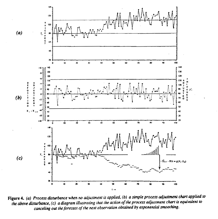
Consider Figure 4(a) which shows 100 observations of the thickness of a very thin metallic deposit taken at equally spaced intervals of time; (see also Box 1991 a). It is desired to maintain this characteristic as close as possible to die target value T = 80. It is evident that, for this process, major drifts from target can occur and in particular ± 3σ --> esta letra es griega limits calculated from the mean successive range show the process to be badly out of control. Other efforts to stabilize the process having failed, the thickness had to be controlled by manually adjusting what we will call the deposition rate X whose level at time t will be denoted by Xt. Effective feedback adjustment could be obtained by using the manual adjustment chart (Box and Jenkins, 1970) shown in Figure 4 (5). To use it the operator records the latest value of thickness and reads off on the adjustment scale the appropriate amount by which he should now increase or decrease the deposition rate.
For example, the first recorded thickness of eighty is on target so no action is called for. The second value of ninety-two is twelve units above the target corresponding on the left hand scale to a deposition rate adjustment X2 - X1 of -2. Thus the operator should now reduce the deposition rate by two units from its present level. The series that would occur if these adjustments were successively made is shown in Figure 4(b).
It will be seen that the adjustment called for by the chart is equivalent to using the "control equation":
Where it must be noted that the successive recorded thickness values yt shown in Figure 4(b) are the thickness readings which would occur after adjustment; the underlying disturbance shown in Figure 4(a) would, of course, not be seen by the operator. The chart is highly effective in bringing the adjusted process to a much more satisfactory state of control and produces in this example a more than five fold reduction in mean square error.
Three pieces of information used in constructing the chart were:
- a change in the deposition rate X will produce all of its effect on thickness within one time interval.
- an increase of one unit in the deposition rate X induces an increase of 1.2 units in thickness y. The constant 1.2 = 6/5 is sometimes called the gain, it is denoted by g and is a scale factor relating the magnitude of the change in y to that of the change in X.
- study of the uncontrolled disturbance time series of Figure 4(a) showed that it could be effectively forecast one step ahead using exponential smoothing with smoothing constant θ = 0.8.
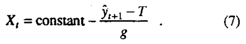
The appropriate* control equation can then be shown to be
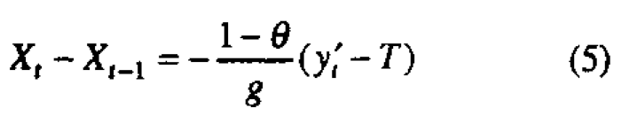
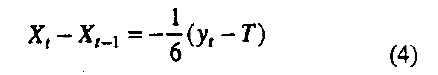
which on substitution yields equation (4). After summation equation (5) may be written
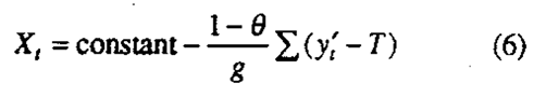
which is the discrete form of what the control engineer calls "Integral Control" action. It may also be shown that this control action is equivalent to
*If the series is such that exponential smoothing with θ = 0.8 produces a minimum mean square error forecast (see for example Box and Jenkins 1970) this control equation will produce minimum mean square error control about the target value.
This says that continual adjustment of the level of the deposition rate Xt must be such as will just cancel out that part 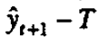 of the disturbance that is predictable by exponential smoothing at time t. Figure 4(c) illustrates this and the vertical arrow indicates the situation for: t = 86
The chart of Figure 4(b) requires that an adjustment be made after each observation. Such charts are of value when the cost of adjustment is essentially zero. This happens, for example, when making a change consists simply of the turning of a valve by an operator who must be available anyway. in other situations, however, process adjustment may require the stopping of a machine or the changing of a tool or some other action entailing cost and it may then be necessary to employ a scheme which calls for less frequent adjustment in exchange for a small increase in process variation.
It was shown by Box and Jenkins (1963), (see also Box, Jenkins and MacGregor, 1974), that this objective can be achieved efficiently with what I will call a bounded adjustment chart which again employs an exponentially weighted average of past data to estimate the deviation to be compensated but calls for only periodic adjustment. The chart is superficially similar to that proposed for process monitoring by Roberts (1959). However, the location of the limit lines for bounded adjustment charts are not chosen to detect statistically significant deviations but rather to balance a reduction in the frequency of needed adjustment against an acceptable increase in the standard deviation of the adjusted process. They are typically much narrower than those used for process monitoring.
Figure 5 shows such a bounded adjustment chart for the first fifty values of the thickness data used for illustration in Figure 4(a). The open circles represent the observations  of thickness which would be obtained after adjustments had been made by periodically changing the deposition rate
  . The filled circles
  are forecasts made one period previously using the appropriate exponentially weighted average. The estimated value of θ used in calculating the EWMA is as before 0.8. The forecasts
  are updated by the well known formula
  . The particular chart shown in Figure 5 has boundary lines at T ± 8 where T = 80 the target value. This results in the average frequency of needed adjustments being reduced to once in every fourteen intervals at the expense of increasing the mean square error by about 18%. A table showing the frequency of needed adjustment and the corresponding increase in mean square error associated with a widening and narrowing of the limit lines is given in Box (1991b). Adjustment charts or the kind described here can be shown to have optimal properties on plausible assumptions fully set out in the original derivations referred to above. Recent computer simulations have shown however that these charts are remarkably robust to changes in the model. Indications are that they work remarkably well under a wide range of conditions.
Statistical Experimental Design
The invention in the 1920's by Fisher of experimental design is a landmark in human progress. He showed for the first time how experiments can be conducted which were logically valid and statistically efficient. Today these ideas play a major role in switching from the outdated philosophy of attempting to inspect bad quality out to the modem concept of building good quality in. Unfortunately, in the present teaching of experimental design some of its most fundamental aspects seem to be often overlooked. This is possibly because of a basic misunderstanding by some teachers of statistics about the relative importance of empirical science and theoretical mathematics. For illustration, I will describe how we introduce at my university the basic ideas of experimental design in a short course (lasting a week or less) for scientists and engineers (see Box 1991c).
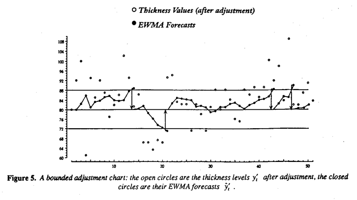
For this purpose, we will find it very valuable to use a paper helicopter for illustration. We were introduced to this idea some years ago by Kip Rogers of Digital Equipment. Using the generic design shown in Figure 6, a "helicopter"; can be made from an 8 1/2 x 11 sheet of paper in about a minute or so. The scenario I'll describe requires three people who I'll call Tom, Dick, and Mary. To make an experimental run, Tom stands on a ladder and drops the helicopter from a height of twelve feet or so while Dick times its fall with a stopwatch. We explain to the class that we would like to find an improved helicopter design which has a longer flight time. The helicopter can then be used to illustrate a number of important ideas.
Variation
We start by Tom dropping a helicopter made from blue paper. He drops it four times and we see that the results vary somewhat. This leads to a discussion of variation and to the introduction of the range and the standard deviation as measures of spread, and of the average as a measure of central tendency.
Comparing Mean Flight Times
At this point Dick says "I don't think much of this helicopter design, I made this red helicopter yesterday and dropped it four times and I got an average flight time which was considerably longer than what we just got with the blue helicopter." So we put up the two sets of data for the four runs made with the blue helicopter and the four runs made with the red helicopter, on the overhead projector and we show the two sets of averages and standard deviations. Eventually we demonstrate a simple test that shows that there is indeed a statistically significant difference in means, in favor of the runs made with the red helicopter.
Validity of the Experiment
At this point Mary says "So the difference is statistically significant. So what? It doesn't necessarily mean it's because of the different helicopter design. The runs with the red helicopter were made yesterday when it was cold and wet, the runs with the blue helicopter were made today when it's warm and dry. Perhaps it's the temperature or the humidity that made the difference. What about the paper? Was it the same kind of paper used to make the red helicopter as was used to make the blue one? Also, the blue helicopter was dropped by Tom and the red one by Dick. Perhaps they don't drop them the same way. And where did Dick drop his helicopter? I bet it was in the conference room, and I've noticed that in that particular room there is a draft which tends to make them fall towards the door. That could increase the flight time. Anyway, are you sure they dropped them from the same height?" So we ask the class if they think these criticisms have merit and they mostly agree that they have, and they add a few more criticisms of their own. They may even tell us about the many uncomfortable hours they have spent sitting around a table with a number of (possibly highly prejudiced) persons arguing about the meaning of the results from a badly designed experiment.
We tell the class how Fisher once said of data like this that "nothing much can be gained from statistical analysis; about all you can do is to carry out a postmortem and decide what such an experiment died of." And how, some seventy years ago, this led him to the ideas of randomization and blocking which can provide data leading to unambiguous conclusions instead of an argument. We then discuss how these ideas can be used to compare the blue and the red helicopter by making a series of paired comparisons. Each pair (block) of experiments involves the dropping of the blue and the red helicopter by the same person at the same location; you can decide which helicopter should be dropped first by, for example, tossing a penny. The conclusions are based on the differences in flight time within the pairs of runs made under identical conditions. We go on to explain however that different people and different locations could be used from pair to pair and how, if this were done "it would widen the inductive basis" as Fisher (1935) said, for choosing one helicopter design over the others if the red helicopter design appeared to be better, one would, for example, like to be able to say that it seemed to be consistently better no matter who dropped it or where it was dropped. As we might put it today, we would like the helicopter design to be "robust with respect to environmental factors such as the 'operator' dropping it and the location where it was dropped." This links up very nicely with later discussion of experimental methods for designing products that are robust to the environment.
Simple factorial experiments which Fisher introduced are of great importance to quality line improvement because of their very high statistical efficiency and their ability to detect and estimate interactions. A good illustration of the enormous power of even and extremely simple design was demonstrated for example by Hellstrand (1989) who is employed by SKF, one of the largest manufacturers of ball bearings with plants in fourteen different countries. The bearing under investigation is shown in Figure 7(a). Figure 7(b) shows a simple factorial design in three variables-heat treatment, outer ring osculation, and cage design-each at two levels. The numbers show the relative lengths of lives of the bearings. If you look at Figure 7(b), you can see that the choice of cage did not make a lot of difference. (This itself was an Important discovery which conflicted with previously accepted folklore and led to considerable savings.) But, if you average the pairs of numbers for cage design you get the picture in Figure 7(c), which shows what the other two factors did. This led to the extraordinary discovery that, in this particular application, the life of a bearing could be increased fivefold if the two factor(s) outer ring osculation and inner ring heat treatments were increased together. This and similar experiments have saved tens of millions of dollars.
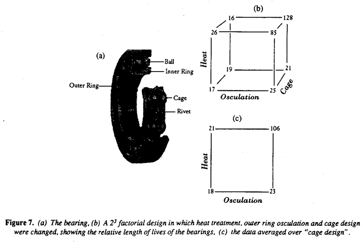
Remembering that bearings like this one have been made for decades, it is at first surprising that it could take so long to discover so important an improvement. A likely explanation is that, because most engineers have, until recently, employed only one factor at time experimentation, interaction effects have been missed. One factor at a time experimentation became outdated 65 years ago with Fisher's invention of modern methods of experimental design, but it has taken an extraordinary long time for this to permeate teaching in engineering schools and to change the methods of experimentation used in manufacturing industry. In the United States the chemical industry and other process industries have long used such methods (although not as extensively as they should) but large portions of industry, concerned with the manufacture of parts, seem only recently to have become aware of them.
But the good news is because of past neglect (a) many important new possibilities that depend on interactions are waiting to be discovered. (b) the means by which such discoveries can be made is simple and readily available to every engineer.
As far as analysis is concerned in this example little more than visible inspection of the data is needed. I'm not saying that more sophisticated methods aren't valuable when properly applied. But I am saying that the basic concepts of experimental design are simple and that we should begin by just getting our engineers to run a simple design like the one above. This will usually whet their appetite for more. Even if a design such as this was the only one they ever used, and even if the only method of analysis that was employed was merely to eyeball the data, this alone could have an enormous impact on experimental efficiency, and the rate of innovation. As with other statistical techniques experimental design can be used:
- widely in elementary form by the general workforce;
- less widely to solve more sophisticated by specially trained engineers and scientists.
Evolutionary Operation
An example of the elementary use of experimental design by the workforce is Evolutionary Operation (Box 1957; Box and Draper 1969). The philosophy is that "a process should be run so as to produce not only product, but also information on how to improve the product". As we've said, passive observation of the day to day running of a process can itself produce information leading to improvement. However, the effect of changes due to altered processes conditions that would never occur in normal operation cannot, of course, be found in this way. In evolution operation, small planned changes which follow a simple pattern are made in the process conditions and constant repetition of this design pattern can lead to continued process improvement.
The general concept is illustrated in Figure 8(a) and a specific example of three phases of Evolutionary Operation leading to a cost reduction of 13% is shown in Figure 8(b) and 8(c). The example is taken from Box, Hunter and Hunter (1978).
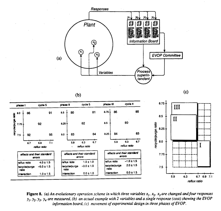
The successful application of Evolutionary Operation, like the application of other quality improvement techniques, requires management interest and involvement which has sometimes been lacking in the West. However, once again, in Japan this technique has been applied with hundreds of successful applications.
In the many more sophisticated uses of Experimental Design different approaches are required at different stages of investigation:
Which variables are important?: Sometimes we may not know which of the number of possible factors are the important ones. At this stage fractional factorial designs and other orthogonal arrays are a great importance fo screening out what Juran has called the vital few factors from the trivial many.
How do they affect response?: Sometimes possibly as a result of screening or because of previous knowledge, the important variables are known but we wish to find out how they affect a particular response or a number of responses. At this stage of experimentation, using factorial designs, mild fractions and response surface methods are important. The models used at this stage are more or less empirical and are often based on polynomials sometimes in suitably transformed variables.
Why do they do what they do?: This stage is less often reached in quality improvement studies it uses mechanistic model building techniques, non-linear least squares and non-liner design.
An Illustration of Screening Factor Using Fractional Design
Fractional factorial design and other orthogonal arrays were developed during and just after WWII in England by Finney (1945), Plackett and Burman (1946) and Rao (1947). The reason for the importance of the designs for screening factors is because of their projective properties. Figure 9(a) shows how a half fraction of a 23 factorial in three variables x1, x2, and x3 has full 22 factorials as projections. Figure 9(b) shows a sixteen run design used in our engieneer's class to screen for important factors that increase flight time of the papa helicopter. This design in eight factors shown at the top of Figure 9(b) is a 1/16 fraction of the four 28 (256 run) design. It projects into a duplicated 2 factorial in every sub-space of three dimensions so that if only up to three factors are of importance, the design will produce a complete 23 factorial design replicated twice in those three factors no matter which ones they are. This latter property is particularly remarkable when we consider that there are fifty-six different ways of choosing three factors from eight.
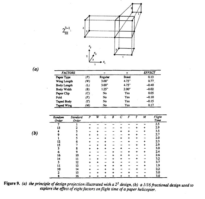
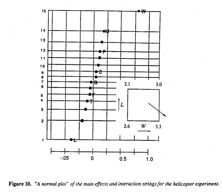
Flight times for the sixteen helicopter types obtained from an experiment run in random order are also shown. From these flight times, terms of the inset diagram in Figure 9(c). The averages of each set of four runs associated with the various conditions of W and L are set out at the corners of the square in the inset diagram. A direction in which one might expect than still longer flight times could be obtained by using larger wings with a shorter body is indicated by the arrow. Thus the experiment immediately provides not only an improved helicopter design but also indicates the direction in which further experimentation should be carried out and so demonstrates the value of the sequential approach to experimentation - learning as you go.
No elaborate analysis is needed for two-level experiments of this kind and certainly no Analysis of Variance table, which at this stage and for this purpose serves only to waste time and confuse engineers and other technologists. Instead we find that the rationale of Daniel's normal plot can readily be explained and is all that is needed.
Response Surface Methods
Some useful properties of Response Surface Methods are that they allow:
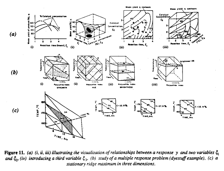
- visualization of relationships between one or more responses and a number of factors de tennining experimental conditions as is illustrated in Figure 11(a).
- the finding and exploiting of optima - a discussion of this application will be found in the original pain by Box and Wilson (1951) and in various books on these methods.
- the study of multiple response problems - Figure 11 (b) shows an example from Box and Draper (1986) of a study of manufacturing conditions of a chemical dye. Of six original factors only three (time, temperature, and polysulfide index) were found to effect the strength, hue and brightness of the dye. The desired condition of hue = 20, brightness = 26, arid maximum strength can be found as indicated in Figure 11(b iv)
- exploitation of ridge systems - it is not sufficiency realized that well conditioned point maxima in responses such as yield and cost are exceptional. More frequently systems are dominated by stationary or rising ridges which arise because of interaction between the factors. An extreme case found for an autoclave process is shown in Figure 11(c). Such ridge systems can be exploited to allow optimization or near optimization of more than one response.
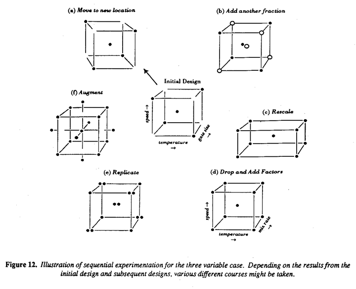
- the use of sequential exploration: At the beginning of an investigation the experimenter knows least about the identity of the important variables, the location of the experimental region of interest, the appropriate scaling and transformation of the variables, the degree of sophistication required to model the system and so forth. Thus "once shot" experimentation which attempts to cover all bases with a single large experiment planned at the beginning of the investigation is likely to be extremely inefficient. Whenever possible sequential experimentation with associated sequential assembly of design (see Fig. 11(d)) which builds on the information supplied by the data as it is obtained much more efficient for industrial experimentation.
Objectives Of Experimental Design
Experimental design can have different objectives among these are:
- to raise the mean value of some quality characteristics
- to reduce the variance
- to find a set of conditions which in some sense produce a robust product in process.
Designing For Robustness
Like most good statistical ideas, designing for robustness has a considerable history. Thus in the early part of this century, Gosset (1958), whose product was the barley to be used by the Guinness brewery, emphasized that experiments should be run in different areas of Ireland so as to find varieties and conditions which were insensitive to particular local environments. Later Fisher (1935) spoke of the "wider inductive basis" for conclusions obtained by comparing treatments under conditions which were different rather than similar. Youden (1961 a,b) and Wernimont (1977) described methods using fractional factorials for designing analytical procedures which have the property of "ruggedness" so that they would give similar results when conducted in different places and by different people. Also the food industry over many years has conducted "inner and outer array" experiments to obtain products such as boxed cake mixes which are insensitive to deviations by the user from the instructions on the box.
The concept that Taguchi (1986) has called parameter design has many aspects. Among these are:
- Robustness to environmental variables,
- Robustness of an assembly to transmitted variation,
- Achieving smallest dispersion about a desired target level,
- An implied experimental strategy.
Robustness To Environmental Variables
To solve these problems Taguchi suggested the use of a cross product experimental arrangement consisting of an "inner" or design array containing n design configurations and an "outer" or environmental array containing m environmental conditions. The environmental conditions could represent variation accidently induced by the system, as in the well known tile experiment of Taguchi and Wu (1985). Alternatively, designated changes might be deliberately induced and suitably arranged in some specific design.
An important problem is that of reducing the amount of effort needed in such a study. Three possibilities are as follows:
- extreme conditions: for the environmental array it is sometimes possible to pick out a smaller number of environmental conditions expected to be extreme and run only these. This method is always risky. When there are many environmental factors, guessing "extreme conditions"; may become difficult or impossible.
- including design and environmental variables in a single design: a possible alternative is to abandon the idea of a cross product design and simply consider the design variables and the environmental variables together as factors in a single design. Questions then arise as to what the structure of this experimental design should be. In particular, what "effects" of the design and environmental factors (linear, quadratic, interaction, etc.) it is important to estimate and how to choose experimental designs to achieve this. Two approaches are those of Shoemaker et al (1990) and Box and Jones (1990a).
- Spin Plotting: When robustness experiments are carried out using cross product designs it is frequently most convenient to conduct them in a split plot mode. In particular, examples described by Phadke et al (1983) arid by Shoemaker et al (1990) are clearly of this type. The concept of designing products that were robust to environmental factors and the value of split plot experiments in achieving this was well understood almost three decades ago by Michaels (1964). He described these ideas in the example from detergent testing at Proctor and Gamble Ltd. U.K. In particular he says:
Environmental factors, such as water hardness and washing techniques, are included in the experiment because we want to know if our products perform equally well vis-a-vis competition in all environments. In other words, we want to know if there are any Product × Environment interactions. Main effects of environmental factors, on the other hand, are not particularly important to us. These treatments are therefore applied to the Main Plots, and are hence not estimated as precisely as the Sub-plot treatments and their interactions. The test products are of course applied to the Sub-plots."
Conducting the designs as split plots or as strip blocks does not change the number m × n of cells in the design but it does change the appropriate analysis and, more importantly, can greatly change the amount of experimental effort required see for example Box and Jones, 1990(b).
Robustness To Error Transmission
In the design of an assembly, such as an electrical circuit, the exact mathematical relation y = ƒ(x) between the quality characteristic of the assembly, such as the output voltage y of the circuit, and the characteristics x of its components (resistors, capacitors, etc.) may be known from physics. However, there may be an infinite variety of configurations of x that can give a working assembly, for example, that can produce a desired mean value E(y) = η. An opportunity therefore exists to choose a configuration which is least affected by variation in the components.
Using a Wheatstone bridge circuit for illustration, Taguchi and Wu (1985) again employ an experimental design strategy using inner and outer arrays. Box and Fung (1986) pointed out, that the effect of variation in the component can be computed by well known error transmission formulae and minimized using a standard optimization program or equivalently by response surface methods. For an early example of using error transmission formally for the study of variability in engineering designs see Morrison (1957) who remarks:
"Most engineering design is based to a large extent on relations between mean values or target values of the design parameters. For a statistical formulation each equation of mean values should be supplemented by an equation in terms of the variance of the design parameters. This will require a knowledge of the component variances, which should be based on actual measurements rather than on guesswork."
The warning in the last sentence is particularly apt because procedures for choosing a robust product can be very unrobust from a statistical point of view Fung 1986 see also Box (1991d). In particular wildly different results can be obtained if, as is in the Wheatstone bridge experiment, for examples a particular error structure assumed to apply over very wide ranges of the x's fails to hold. Also, although for an electrical circuit it is reasonable to assume that the relation y =ƒ(x) is known, when, as is more usually the case, it must be estimated experimentally the problems are much more complicated and require further study.
Achieving Smallest Dispersion About A Defined Target Value
When a dispersion measure of some characteristic y is under study there are advantages in conducting the analysis in terms of the logarithm of the dispersion. In particular (see Bartlett and Kendall, 1946) the transformation log s2(y) stabilizes the variance of the dispersion measure s2(y). In the simulianeous analysis of location and dispersion, Taguchi uses for a dispersion measure the signal to noise criterion SNT = constant log  which is closely approximated by -log s2 (log y).
The reason for, in effect, logging the data before computing the dispersion is (see Phadke 1982) that it is believed that this data transformation is likely to decouple dispersion and location, effects and so to simplify finding those conditions which simultaneously locate the process on target and minimize dispersion about the target. However, a better alternative (Box 1988) is to evaluate a range of transformations which might include the log as a special case (and no transformation as another special case) and carry out the analysis in terms of that transformation which yields maximum simplification.
Experimental Strategy
Taguchi's procedures seem intended only to pick the "optimum" factor combination from a one-shot experiment. Although the immediate object may be this, the ultimate objective must surely be to better understand the engineering system. To do this requires, I believe, efficient statistical tools of design and analysis which accommodate the naturally iterative process of scientific method I have referred to above.
The Importance Of Quality Improvement:
With every day that passes there are more people in this world. More people to provide for, more people who want a decent life. The manner in which organizations have in the past been run, has led to a world where many people are hungry and without jobs. Even in the industrialized countries, for many, the world is one which projects a continuous suggestion of their own worthlessness. We are faced with increasing alienation, mental illness, and turning to drugs and crime.
The quality revolution that I have described of fers great hope because it can provide for everyone:
- a solution to economic problems;
- the possibility of improvement in the quality of life:
- freedom to experience the joy of creativity.
Acknowledgement
This research was sponsored by the National Science Foundation under Grant No. DDM-8808 138.
References
- Box, G.E.P. and Wilson, K. B. (1951), On the Experimental Attainment of Optimum Conditions. Journal of the Royal Statistical Society.
- Box, G.E.P. (1957), Evolutionary Operation: A Method for Increasing Industrial Productivity. Applied Statistics, 6,81-101.
- Box, G.E.P. and Jenkins, G.M. (1963), Further Contributions to Adaptive Optimization and Control: Simultaneous Estimation of Dynamics: Non-Zero Costs. Bulletin of the International Statistical Institute, 34th Session, Ottawa.
- Box, G.E.P. and Draper, N.R. (1969), Evolution Operation: A Statistical Method for Process Improvement, Wiley.
- Box, G.E.P., Jenkins, G.M. and MacGregor, J.F. (1974), Some Recent Advances in Forecasting and Control, Part II. Journal of the Royal Statistical Society, Series C (Applied Statistics. 23),No.2, 158-179.
- Box, G.E.P. and Jenkins, G.M. (1976), Time Series Analysis: Forecasting and Control. Holden-Day, San Francisco, 433-446.
- Box, G.E.P., Hunter, W. G. and Hunter, J.S. (1978), Statistics for Experimenters. New York: John Wiley and Sons.
- Box, G.E.P. and Draper, N.R. (1986), Empirical Model-Building and Response Surfaces. New York: Wiley.
- Box, G.E.P. and Fung C.A. (1986), Studies in Quality Improvement: Minimizing Transmitted Variation by Parameter Design. Report No.8, Center for Quality and Productivity Improvement, University of Wisconsin-Madison.
- Box, G.E.P., (1988), Signal-to-Noise Ratios, Performance Criteria and Transformations. Technometrics 30, 117.
- Box, G.E.P., and Jones, S. (1990a), Designing Products that are Robust to the Environment. Report No.56 Center for Quality and Productivity Improvement, University of Wisconsin-Madison. Submitted to the Journal of Applied Statistics.
- Box, G.E.P., and Jones, S. (1990b), Split-Plot Designs for Robust Product Experimentation. Report No. 61. Center for Quality and Productivity Improvement, University of Wisconsin-Madison. Journal of Applied Statistics (to appear).
- Box, G.E.P. (1991a), Feedback Control by Manual Adjustment. Quality Engineering, 4(1), 143- 151.
- Box, G.E.P. (1991b), Bounded Adjustment Charts, Quality Engineering, 4(2), 333-340.
- Box, G.E.P. (1991c), Teaching Engineering Experimental Design with a Paper Helicopter. Quality Engineering, (to appear).
- Box, G.E.P. (1991d), Contribution to the Discussion: "Taguchi's Parameter Design". Technometrics, (to appear).
- Finney, D.J. (1945), Fractional Replication of Factorial Arrangements. Annals of Eugenics, 12, 291-301.
- Fisher, R.A. (1935), The Design of Experiments. Oliver and Boyd, London and Edinburgh.
- Fuller, F.T. (1986), Eliminating Complexity From Work: Improving Productivity by Enhancing Quality. Report No. 17, Center for Quality and Productivity Improvement, University of Wisconsin-Madison.
- Fung, C.A. (1986), Statistical topics in off-line quality control, Ph.D Thesis, UW Madison.
- Gosset, W.S. (1986), Student's collected papers, Cambridge, Published by the Biometrika Trustees.
- Hellstrand, C. (1989), The Necessity of Modern Quality Improvement and Some Experience. With its Implementation in the Manufacture of Rolling Bearings. Phil. Trans. Royal Society London A, 327,529-537.
- Imai, M. (1986), Kaizen, Random House, New York.
- Ishikawa, K. (1976), Guide to Quality Control. Asian Productivity Organization.
- Juran, J.M. (1988), Juran's Quality Control Handbook. McGraw Hill, New York.
- Michaels, S.E. (1964), The Usefulness of Experimental Design, Applied Statistics, 13, No. 3, 221.228.
- Morrison, S.J. (1957), The Study of Variability in Reprinted in Engineering Design, Applied Statistics, 6, No. 2, 133-138.
- Nair V.N. (1986), Testing in Industrial Experiments with Ordered Categorical Data. Technomerrics, 28,283-291.
- Phadke, M.S., Kackar, R.N., Speeney, D.V., and Grieco, M.J. (1983), Off-Line Quality Control in Integrated Circuit Fabrication Using Experimental Design. The Bell System Technical Journal, 62, 1273-1310.
- Placket, R.L. and Burman, J.P. (1946), The Design of Optimum Multifactorial Experiments. Biometrika, 33,305-325.
- Roberts, S.W. (1959), Control Chart Test Based on Geometric Moving Averages. Technometrics, 1, No.3,239-250.
- Shoemaker, AC., Tsui, K.L., and Wu, C.F.J. (1990), Economical Experimentation Methods for Robust Parameter Design. Submitted for publication.
- Taguchi, G. and Wu, Y. (1985), Introduction to Offine Quality Control. Nagaya Japan: Central Japan Quality Control Association.
- Taguchi, G. (1986), Introduction to Quality Engineering. Asian Productivity Organization, UNIPUB, White Plains, New York.
- Wernimont, G. (1977), Ruggedness Evaluation of Test Procedures. Standardization News, 5, 13-16.
- Youden, W.J. (1961a), Experimental Design and ASTM Committee. Materials research and standards, 1,862-867, Reprinted in Precision Measurement and Calibration, Special Publication 300, National Bureau of Standards, Vol. 1, 1969, Editor H.H. Ku.