Product Design with Response Surface Methods

An Illustration of the Use of Scientific Statistics for Adaptive Learning

Report No. 150
by George Box and Patrick Liu
Copyright © 1998, Used by Permission

Abstract

In this article, methods for demonstrating the iterative process of investigation are presented. As one example, it is shown how the sequential use of response surface techniques may be applied to devise an improved paper helicopter design with almost twice the flight time of its original prototype. The purpose of this paper is to demonstrate the process of investigation and how it can be catalyzed by the use of statistics. Although individual designs and analyses are used these are the "trees" behind which we hope the forest will be clearly visible.

Keywords: Iterative Investigation, Response Surface Methods, Sequential Assembly, Paper Helicopter, Design of Experiments, Steep Ascent Methods, Ridge Analysis

Introduction

By the late 1940's earlier attempts to introduce statistical design at a major division of ICI in England using large preplanned all-encompassing experimental designs had failed. The "one-shot" approach with the experimental de sign planned at the start of the investigation when least was known about the system was clearly inappropriate. In this industrial environment, results from an experiment were often available within days, hours, or sometimes even minutes. Advantages offered by this greater immediacy could he realized only by a philosophy of experimentation suited to the process of adaptive learning in which ideas were modified as experimentation progressed - philosophy which the skilled industrial investigator would naturally use. Response Surface Methods (Box and Wilson, 1951) were developed as one means of filling this need (see also Daniel, 1962).

Unfortunately, the one-shot experiment, where all aspects of the problem - the appropriate factors to be studied, the appropriate region in which to experiment, the form of model to be fitted and so forth - are all assumed known in advance, has received almost undivided attention by researchers and teachers in statistics. This is presumably because that form of experiment can be conveniently fitted into a fixed mathematical framework, within which, theorems can be proved and researchers, can develop "optimal" decision procedure, "optimal" experimental designs and so forth.

Although in some experimental trials the one-shot approach is necessary (for example in many medical trials), such trials form only a very small part of the body of experimentation needed in research and development. Consequently, statisticians limited to this static mind-set have usually been found to be a hindrance rather than a help to adaptive learning and have thus excluded themselves from an enormous and comparatively unexplored field where statistical methods appropriate to changing rather than to static ideas could be of enormous help. Unfortunately, many researchers and teachers in statistics have similarly hobbled their own activities. To rigorously explore the consequences of supposedly available knowledge is, of course, an essential part of scientific investigation, but what is paramount is the discovery of new knowledge. There is no logical reason why the former should impede the latter but this is what has happened.

Since the time of Aristotle it has been known that the generation of new knowledge occurs as a result of deductive-inductive iteration. Aristotle's concept was developed and restated by Grosseteste in the thirteenth century and later by Francis Bacon, and is inherent in the Shewhart-Deming cycle for continuous quality improvement. It is a necessary theme for any serious discussion of scientific investigation.

In this context of adaptive learning, it is recognized that the appropriate factors to be studied, the regions of interest in the factor space, the form of the models to be fitted and so forth must all initially be guessed by the investigator and as s/he learns more about them, and that they will almost invariably change. Thus for adaptive learning one cannot hope to produce a rigid and unique "optimal" procedure. What can be done is to develop techniques which when used in cooperation with the investigator, can catalyze a process of iterative learning that can be used by different investigators, start from different places and follow different routes and yet have a good chance of converging on some satisfactory solution when such exists. In this paper we illustrate such a process using iterative statistical methods to improve the design of a paper helicopter.

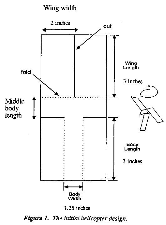
The prototype design for a paper helicopter, shown in Figure 1, was kindly made available to us by Kipp Rogers of Digital Equipment Corporation. The objective of our experiment was to find an improved helicopter design giving consistently longer flight times. Our test flights were carried out in a room with a ceiling 102 inches (8' 6") from the floor. The wings of each tested helicopter were initially held against the ceiling and the flight time was measured with a digital stop watch.

Design I: An Initial Screening Experiment

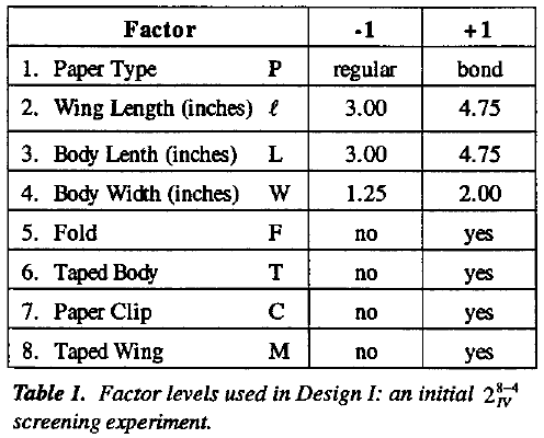
After considerable discussion it was decided to begin by testing the eight factors (input variables) each at two levels listed in Table 1 and with plus and minus limits shown there. The response (output variable) was the flight time. The initial experimental plan defined sixteen helicopter types set out in Table A.1. (In general, the letter A before a table or figure means that the table or figure will be found in the Appendix.) The experimental design is a fractional factorial (see for example Box et al, 1978). Each of the sixteen types of helicopter was dropped four times and the flight times recorded in centiseconds (units of one hundredth of a second). The mean flight times and the standard deviations are also shown in the Table A.1 together with the quantity 100 log s which we will call the dispersion. It is well known (Bartlett and Kendall, 1946) that for the analyses of variation there are considerable advantages in using the logarithm of the sample standard deviation s rather than s itself. To avoid decimals, we have used 100 log s in our analysis and we refer to this quantity as the dispersion. The effects calculated from the mean flight time will be called location effects. Effects calculated using the dispersion 100 log s will be called dispersion effects. Visual observation suggested that larger variation of flight times was usually associated with in stability of the helicopter design.

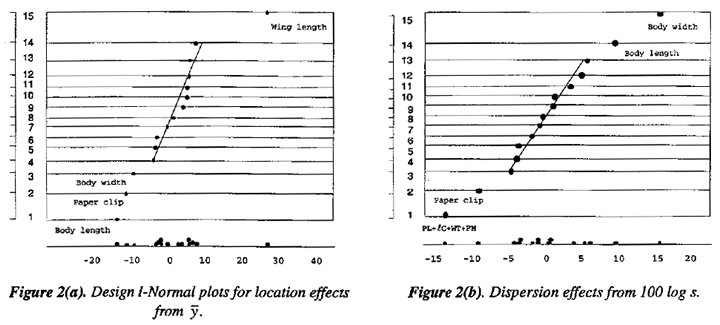
The effects are shown as regression coefficients thus the constant term is the overall average and each of the remaining coefficients is one half of the usual factor effect. Normal plots for these effects are shown in Figure 2(a) and (b). Figure 2(a) for location effects shows that factors describing three of the dimensions of the helicopter - wing length , body length L, and body width W - all have distinguishable effects on mean flight time but that of the five remaining "qualitative" variables only factor C (corresponding to the application of a paper clip to the body of the helicopter) is appreciable and is negative.

The plot for dispersion effects in Figure 2(b) shows effects for wing length , body length L, body width W, paper clip C and for the string of interactions 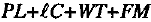. Also, the signs of the coefficients are such that changes in the dimensional variables , L, and W, which gave increases in the mean flight time, were also associated with reductions in dispersion. However the addition of a paper clip, while reducing the dispersion, also decreased the flight time. We made a judgment that for the moment we would concentrate on increasing flight times and not use the paper clip. We could reconsider this later if instability became a problem. Also, we decided that we would not attempt to interpret or to separate out by additional runs, the interaction string at this time.

On this basis a linear model for estimating mean flight times in the immediate neighborhood of the experimental design was

where the coefficients are those in Table A.1 suitably rounded.

Equation (1) is usually called a linear regression model since the coefficients 223, 28, -13, and -8 are those that would be obtained by fitting the equation by least squares.

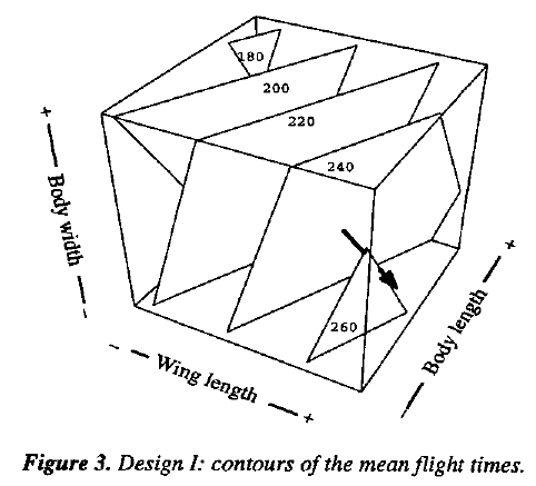
The contour diagram of Figure 3 is a convenient way of conveying visually what is implied by Equation (1). For example, the equation implies that combinations of x₂ , x₃, and x₄ on the 240 contour plane should all produce alternative helicopter designs with flight times of about 240 centiseconds.

Steepest Ascent Using the Results from Design I

Now, since increasing the wing length l and reducing the body length L and body width W all had a positive effects on mean flight time, it might be expected that helicopter design with greater wing lengths and with reduced body lengths and body widths might give even longer flights. We can determine such helicopter designs by exploring the direction at right angles to the contour planes indicated by the arrow in Figure 3. In the units of x₂, x₃, and x₄ this is the direction of greatest increase at a given distance from the design center and is called the direction of steepest ascent.

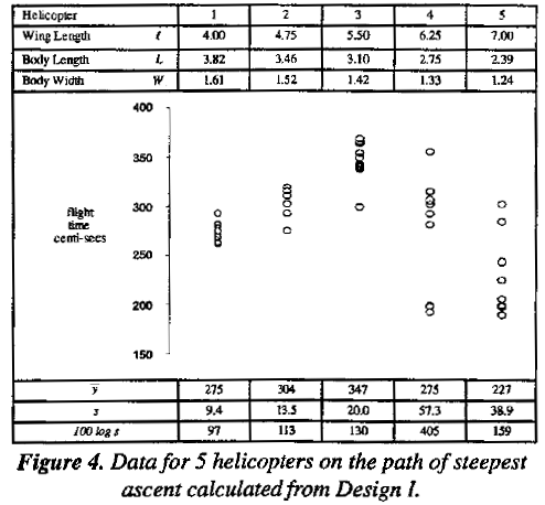
To calculate a series of points along the direction of steepest ascent you don't need a contour plot. You can do this by starting at the center of the design and changing the factors in proportion to the coefficients of the fitted equation. Thus the relative changes in x₂, x₃, and x₄ are such that for every increase of 28 units in x₂, x₃ is reduced by 13 units, and x₄ by 8 units. The units are the scale factors s_t = 0.875, s_L = 0.875, and s_w = 0.375 which are the changes in , L, and W corresponding to a change of one unit in x₂, x₃, and x₄ respectively.

In our investigation we chose the first point P₁ to give a helicopter with a 4 inch wing length and we then increased by 3/4 inch increments adjusting the other dimensions accordingly. This produced the designs corresponding to P₂, P₃, P₄, and P₅ shown in Figure 4. Experiments along such a path can be run sequentially and the spacing of the points along the path can be made a matter of judgment guided by results as they occur. For example, you might have decided to take a large jump initially and try the design P₅ right away. This would have given a disappointingly low result causing you to back track and perhaps to test P₂ or P₃ next. In our investigation we ran experiments in sequence at all the five points making ten repeat drops at each point. As you see from Figure 4, P₃, gave the longest average flight time of 347 centiseconds - the best result obtained so far. Further exploration along this path (designs P₄ and P₅) gave lesser mean flight times and higher standard deviations.

Since none of the qualitative variables we tried in this and previous experimentation (including heavy paper, fold at the wing tip, fold at the base, etc.) seemed to produce any positive effects we decide to fix the overall features of the design and explore more thoroughly the effects of the dimensional variables - wing length , wing width w, body length L, and body width W using a full factorial experiment.

Design II: A Factorial Experiment in Wings and Body Dimensions.

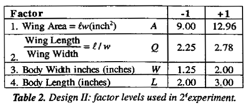
At about this time discussion with an engineer led to the suggestion that a better way to characterize the dimensions of the wing might be in terms of wing area , and length to width ratio . In subsequent experimentation this reparameterization was therefore adopted.

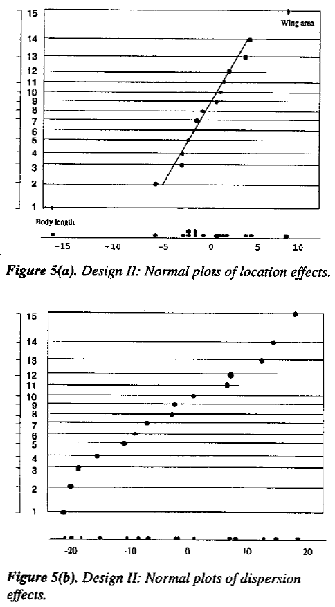
A 2⁴ factorial in the four dimensional variables A, Q, W, L centered close to the previous best conditions is set out in Table 2. Data are given in Table A.2. The normal plot for mean flight times in Figure 5(a) showed large location effects for wing area A and body length L but that for dispersion did not show any evidence of real effects. It was decided, therefore, to try to gain further improvement of fight times by using steepest ascent based on the two large effects using the model

where x₁ and x₄ are recoded variables for wing area (A) and body length (L), respectively.

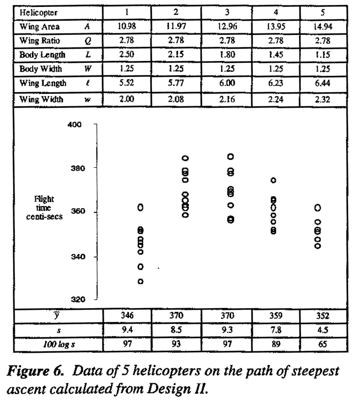
The path was explored by making ten drops at each of five different conditions set out in Figure 6. Interpolation suggests that the best design along this path required wing Area A to be about 12.4 and body length about 2.0 at which the average flight time was 370 centiseconds - a further valuable improvement. It is also worth noting that the dispersions for the five tested helicopters on this path were not large and these helicopters were extremely stable.

After this investigation had been completed a review of the results showed that the path of ascent had been slightly miscalculated. The relative changes in x₁ and x₄ which should have been 8:17 but were mistakenly taken to be 8:11. This rather minor deviation is unlikely to have made much difference. It is worth noting the error we made arose from accidentally switching certain experimental runs. It underlines the importance of checking and rechecking experimental procedures. It also illustrates that in an iterative scheme of this kind, errors tend to be self-correcting.

Design III: A Sequentially Assembled Composite Design

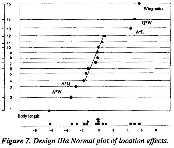
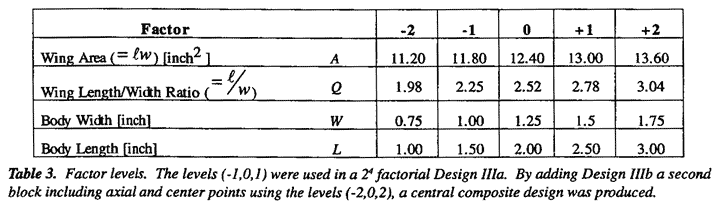
The (-1, 0, 1) levels shown in Table 3 were now used in a further 2⁴ factorial arrangement in the factors A, Q, W L referred to as Design IIIa. This was centered around the best point so far reached. The results are shown in Table A.9. It seemed likely at this stage of the investigation that further advance with first order steepest might not be possible and that a hill second degree equation might be needed to represent the flight times in the new experimental region that had been reached. This was not certain however, so a new 24 factorial experiment in A, Q, W, and L was run with two added center points. Depending on the results obtained, this could become the first block of a second order composite design. The analysis for Design IIIa is shown in Table A.4 and the normal plot for the mean flight times is shown in Figure 7. The corresponding plot for dispersion effects failed to show anything of interest and is not given. We see from Figure 7 that, for average flight times some two factor interactions are quite large and approaching the size of certain main effects suggesting that we should add further runs which will allow estimation of the remaining second order (quadratic) terms. A second block was therefore added consisting of eight axial points with four additional center points. This is set out in Table A.3 and referred to as Design IIIb.

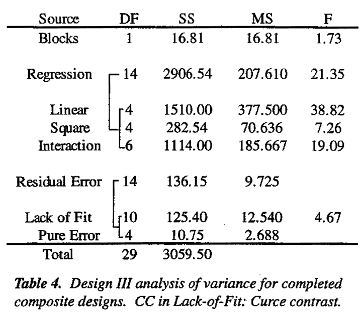
An analysis of variance for the completed design is given in Table 4. There is, somewhat weak, evidence; of lack of fit, nevertheless for this analysis we have used the overall residual mean square of 9.9 as the error variance. The overall F ratio for the fitted second degree equation is 21.35, exceeding its five percent significance level of F_0.05,14,14 = 2.48 by a factor of 8.61. Thus complying with the argument of Box and Wetz (1973) (see also Box and Draper. 1986) that a factor of at least four is needed to ensure that the fitted equation is worthy of further interpretation.

Proceeding further with the analysis we find that the fitted equation is

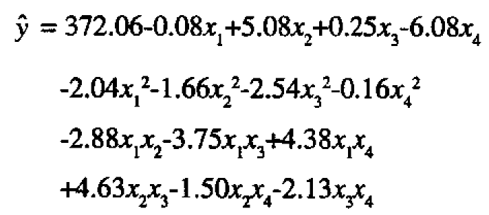
We have shown the constant term and the four linear terms on the first line, the four quadratic terms on the second line, and the six interaction terms on the third and fourth lines. The standard errors for these linear, quadratic, and interaction effects are respectively 0.64, 0.60, and 0.78. This second degree equation in four variables x₁, x₂, x₃, x₄ contains 15 coefficients and in its "raw" form is not easily understood. We briefly review methods of analysis which can make its meaning clear and allow further progress. A fuller account of such analysis is given, for example, in Box and Draper (1987). Here we first illustrate the analysis in Figures 8 and 9 for constructed examples in just two variables x₁ and x₂.

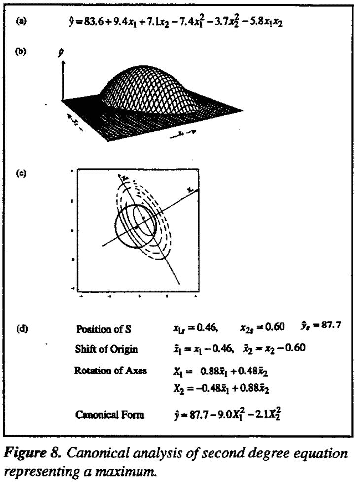
Look at Figure 8. Suppose that in the circle indicated in Figure 8(c) a suitable design has been run centered on the point O (x₁₀ = 0, x₂₀ = 0) yielding the second degree equation shown in 8(a). Figure 8(b) shows a computer plot of the corresponding response surface wich contains a maximum.

A plot of contours of the surface is shown in Figure 8(c). Contour plots of this kind are very helpful in understanding the meaning of a second degree equation when 38.82 there are only two or three input variables (x) but such methods are not available when there are more input variables. Canonical analysis, however, which we now explain makes it easy to understand the meaning of any fitted second degree equation for any number of such variables. Canonical analysis goes in two steps the mathematics is sketched in Figure 8(d) and illustrated geometrically in Figure 8(c):

1. the origin of measurement is shifted from O to S where S is the center of the contour system (in this case the maximum);
2. the axes rotated about S so that they lie along the axes of the elliptical contours which are denoted by X₁ and X₂.

In this way the quadratic equation of 8(a) is expressed in terms of a new system of coordinates X₁ and X₂ in the simpler form .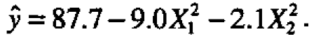

By inspection of this canonical form one can understand the meaning of the quadratic equation without a contour plot. In this case, since the coefficients -9.0 and -2.1 which measure the quadratic curvatures along the X₁ and X₂ axes are both negative, the point S (at which = 87.7) must be a maximum. Also you can see that, if you move away from S in either direction along the X₁, axis, falls off much more rapidly than that if you move similarly along the X₂ axis. Thus you know the contours are drawn out (attenuated) along the X₂ axis which has the smaller coefficient.

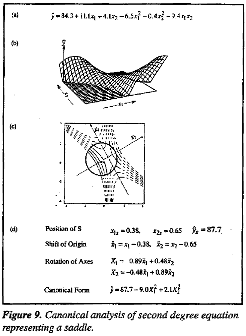
Now look at Figure 9. Equation 9(a) produces the response surface shown in 9(b) which represents a "saddle" or minimax whose contours are shown in 9(c). Again it is easy to understand the nature of the surface without any graphical aid using the canonical form of equation which turns out to be .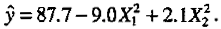

Since the coefficient of is negative and that of is positive, the center of the system S is a maximum as we move along theX₁ axis but is a minimum along the X₂ axis. Thus we know at once that the surface is a minimax. In particular, this implies that movement away from S along the X₂ axis in either direction gives larger values of suggesting the existence of more than one maximum. In response surface studies such saddles are rather rare; but, as we shall see, they can occur.

Analysis for the Helicopter Data

If we apply the canonical analysis outlined above to Equation (3) obtained for the helicopter data we get:

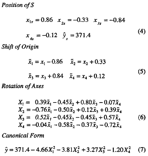
Now we had thought it likely that we would find a maximum at S in which case all four squared terms in (7) would have had negative coefficients. However, the coefficient +3.24 of is positive and its standard error is about 0.61 (roughly the same as that of a quadratic coefficient in Equation (3)). This implies that the response surface almost certainly has a minimum in the direction represented by X₃. If this is so, we will be able to move from the point S in either direction along the X₃ axis and get increased flight times.

Now X₃, expressed in terms of the centered is . Thus beginning at S one direction of ascent along the X₃ axis is such that for each increase in of 0.52 units, must be reduced by 0.45 units, 1, reduced by 0.45 units, and increased by 0.57 units. The units are those of the design given in Table 3. To follow the other direction of ascent you must make precisely the opposite changes. Before we explore these possibilities further, we consider a somewhat different form of analysis.

Ridge Analysis

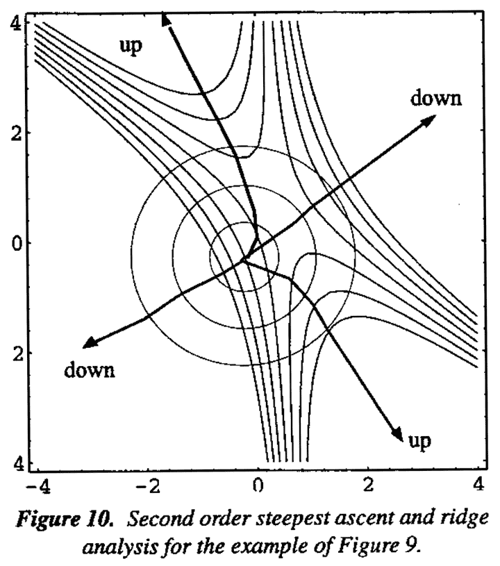
In the original paper by Box and Wilson (1951) the application of the method of steepest ascent to response surfaces was discussed in general and in particular for second degree equations as well as for linear models. For two variables the general concept can be understood by considering again the two dimensional contour representation of the minimax surface in Figure 9(c). As shown in Figure 10 suppose a series of concentric circles are drawn centered at point O with increasing radius r. It can be shown that as the radius r is increased the circles will touch the contours of any response surface at a series of points at which the rate of increase or decrease in response with respect to r will be greatest. In the units of x the path formed by such points is thus one of maximum gradient and hence of steepest ascent or descent. For a first degree equation, such as Equation (1), this is a straight line path at right angle to the planar contour surfaces as in Figure (3). More generally, the path is curved. For a second degree equation, points along the paths of maximum gradient can be found for different values of r by solving a series of linear equations. A. E. Hoerl (1959) developed an extended a technique of this kind under the general heading of Ridge Analysis and illustrated its use with many applications (see also R.W. Hoerl, 1985).

For illustration, Figure 10 shows, for the minimax surface of Figure 9, the paths of maximum gradient (two of steepest ascent and two of steepest descent originating from S.) In this example where O is close to S these paths converge very rapidly onto the axes of the canonical variables X₁ and X₂. Indeed these axes are themselves the path of steepest gradient if we start at S instead of O. For the helicopter example the paths of ascent can be followed either by ridge analysis from the origin O or by following the X₃ axis from the origin S. By either method, we obtained for this example almost identical results.

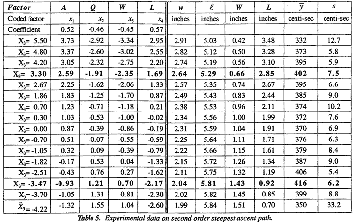
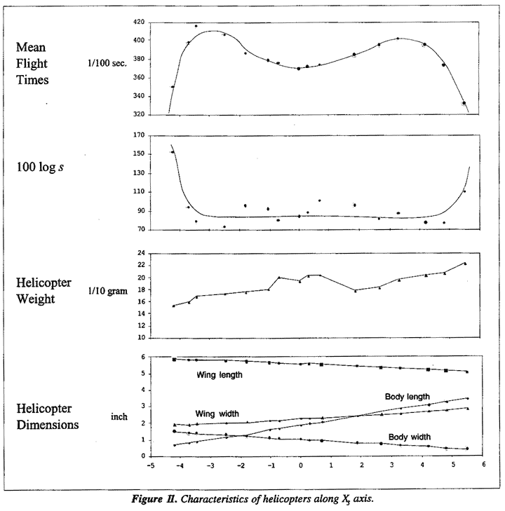
Mean flight times and dispersion for a series of helicopter designs along the X₃ ridge summarized in Table 5. To better understand these results we also show the dimensions of the tested helicopters in terms of the original variables wing length , wing width w, body length L, and body width W.

These tests fully confirm what was implied by the earlier analysis - that we can indeed get a longer flight times by proceeding in either of two directions. Namely by increasing wing width w, body length L and reducing body width W and wing length or by doing precisely the reverse. For sixteen helicopter designs along this path, Figure 11 shows graphically the mean flight times and standard deviations of flight times together with the dimensions of the associated helicopter. It will be seen that in either direction mean flight times of over 400 centiseconds can be obtained. These are almost twice the flight time of original helicopter design. In both directions mean flight times go through maximum. The standard deviations are apparently constant except at the extremes where rapid increase occurred owing to instability.

At this point we decided to stop the present investigation although we fully expect that ways can be found to get longer flight times. We hope that others may be interested in doing this.

Acknowledgment

We are grateful to acknowledge our cooperation with Sandra Martin in early preliminary work on this topic. This work is sponsored by National Science Foundation grant number DMI-9414765.

1. Bartlett, M. S. and Kendall, D. G., "The Statistical Analysis of Variance-Heterogeneity and the Logarithmic Transformation," J. Roy. Statis.Soc., Series B, 8, 128-150, 1946
2. Box, G. E. P. and Wilson, K. B., "On the Experimental Attainment of Optimum Conditions," Journal of the Royal Statistical Society, Series B, 8, 128-150, 1946.
3. Box, B.E.P. and Wetz, J., "Criteria for Judging Adequacy of Estimation by an Approximating Response Function", University of Wisconsin Statistics Department Technical Report No. 9, 1973.
4. Box, G.E.P., Hunter, W. G., and Hunter, J. S., Statistics for Experiments, John Wiley & Son; New York; 1978.
5. Box, G. E. P. and Draper, N. R., Empirical Model-Building and Response Surface, John Wiley & Son; New York, 1987.
6. Daniel, C., "Sequences of Fractional Replicates in the 2^p-q Series," J. Am. Statist, Assoc., 57, 403-429, 1962.
7. Hoerl, A.E., "Optimum Solution of Many Variable Equations." Chem. Eng. Prog., 55, 69 - 78, 1959.
8. Hoerl, A.E., "Ridge Analysis," Chem. Eng. Prog. Symp. Ser., 60, 67-77, 1964.
9. Hoerl, R. W., "Ridge Analysis 25 years later," Am. Statist., 39, 186-192, 1985.