Finding The Active Factors in Fractionated Screening Experiments

R. Daniel Meyer and George Box
Copyright © April 1992, Used by Permission

Also published in Journal of Quality Technology, Vol. 25. No.2. pp. 94-105.

Highly fractionated factorial designs and other orthogonal arrays are powerful tools for identifying important, or active, factors and improving quality. We show, however, that interactions and important factors involved in those interactions may go unidentified when conventional methods of analysis are used with these designs. This is particularly true of Plackett and Burman designs with number of runs not a power of two. A Bayesian method is developed in which the marginal posterior probability that a factor is active is computed and allows for the possibility of interactions. The method can be applied to both orthogonal and nonorthogonal designs as well as other troublesome situations, such as when data are missing, extra data are available or factor settings for certain runs have deviated from those originally designed. The value of the new technique is demonstrated with three examples in which potential interactions and factors involved in those interactions are uncovered.

Introduction

There are many variables that affect a typical process, influencing both location and dispersion. Of the many potentially important variables, it is often the case that only a few are truly important, or active. This is referred to as a condition of factor sparsity (Box and Meyer (1986a, b)). In many situations there is little firm knowledge of exactly which variables are active. A screening experiment is typically carried out to identify the active factors. More extensive experimentation can then focus on these factors.

There are two classes of two-level orthogonal designs most popularly used for screening experiments: the 2^k-p fractional factorials (see, for example, Finney (1945), Box and Hunter (1961)) for which the number of runs is always a power of two; and the two-level orthogonal array designs of Plackett and Burman (1946) for which the number of runs is always a multiple of four. Either of these types of designs can be written as a set of columns of plus and minus signs with an equal number of plusses and minuses in each column. Averaging the observed data opposite the plus signs for a particular column and subtracting the average of the data opposite the minus signs, yields a data contrast. The expected value of a data contrast is called its alias and is a linear combination of various main effects and interactions.

Fractional factorial designs of the type 2^k-p have a relatively simple aliasing structure in which a particular alias term (main effect or interaction) appears only once in association with a single data contrast, with a coefficient which is either 1 or -1. Plackett-Burman designs for which the number of runs is also a power of 2 (8, 16, 32, etc. runs) are called geometric by Plackett and Burman (1946) and are the same designs as the 2^k-p designs. (Any 2^k-p design can be formed by choosing the appropriate columns from the geometric Plackett-Burman design with 2^k-p runs and possibly switching minus and plus signs in some of the columns.) Plackett-Burman designs with number of runs not a power of 2(12, 20, 24, etc. runs) are called nongeometric and have more complicated aliasing relationships than the geometric designs. A particular alias term can occur a number of times associated with a number of different data contrasts and with fractional coefficients. For example, in the 12-run Plackett-Burman design, the data contrast associated with the main effect of any factor has in its alias all two-factor interactions not involving that factor, each with fractional coefficient ±1/3. The general way of obtaining the alias pattern for any design was given by Box and Wilson (1951), and the necessary relationship between the coefficients of the aliases for all orthogonal designs was given, in general, by Box (1952).

Regardless of the design used, the typical approach to analysis is to calculate a set of contrasts, one for each column of the full design array. A variety of different methods may then be applied (normal probability plots, Daniel (1959, 1976); Box, Hunter and Hunter (1978); Bayes plots, Box and Meyer (1986a); pseudo-standard error, Lerith (1989) and others) to identify contrasts which are too large to attribute to noise alone. Identifying active factors then requires associating large contrasts with experimental factors, either as main effects or interactions.

A common strategy in analyzing saturated or nearly saturated experiments is to identify as active those factors whose main effects can be associated with large contrasts, discounting the possibility of interactions. (Indeed, screening designs are often referred to as main-effect plans.) While authors (e.g., Box, Hunter and Hunter (1978)) endorse close examination of the alias relationships of the design when associating large contrasts with experimental factors and in this way accounting for the possibility of interactions, there are a large number of possibilities to consider in this examination of the alias structure. The risk of missing a potential explanation of the data involving interactions seems great when a highly fractionated design is used. For the nongeometric Plackett-Burman designs, the confounding is too complicated to comprehend by visual examination of the alias structure.

A different approach, stemming from the principle of parsimony or in Juran's words, distinguishing the "vital few" factors from the trivial many, supposes that only a small number (perhaps two or three or four) of the factors that are in the design are responsible for most of what is happening, but these active factors may interact with each other. Thus, say, with five factors A, B, C, D and E various hypotheses might be considered. One is that a single factor A, B, C, D or E is responsible for all that is going on, in which case one need only consider the five main effects A, B, C, D and E. Alternatively, on the hypothesis that two factors are responsible, the subset of main effects A and B with interaction AB and the subset of main effects A and C with interaction AC, etc., are possibilities. On the hypothesis that three factors, say A, B and C, may be active, the subset of main effects A, B and C with interactions AB, AC, BC, and ABC are considered together and so on. In the following section we develop a Bayesian method that will more completely consider these various hypotheses when analyzing the results of a screening experiment. The Bayesian model makes it possible to consider all the hypotheses even when the effects are thoroughly confounded, as in Plackett-Burman designs where the alias structure may be quite complicated. In addition, this particular analysis may be applied whether the design is orthogonal or nonorthogorial.

The Model

Our basic approach is to consider all the possible explanations (including interactions) of the data from a screening experiment and identify those which fit the data well. A Bayesian framework is used to give an appropriate measure of fit to each model considered (posterior probability) that can be accumulated in various ways (marginal posterior probability). It is analogous to all-subsets regression in that all models being entertained are evaluated.

The Bayesian approach to model identification is as follows (see, for example, Box and Tiao (1968)). We consider a set of models M₀,..., M_m. Each model M_i has an associated vector of parameters θ_i so that the sampling distribution of data y, given the model M_i, is described by the probability density p(y|θ_iM_i) abajo, ej. The prior probability of the model M_i. is p(M_i), and the prior probability density of θ_i is p(θ_i|M_i). The predictive density of y, given model M_i, is written p(y|M_i), and is given by the expression

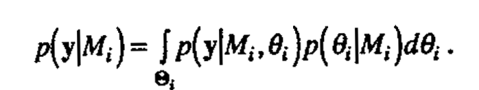
Here Θ_i is the set on which p(θ_i|M_i) is defined. The posterior probability of the model M_i given the data y is then

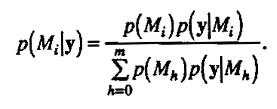
The posterior probabilities p(M_i|y) provide a basis for model identification-tentatively plausible models are identified by their large posterior probability. Computationally we calculate p(M_i)p(y|M_i) for each model M_i and then scale these quantities to sum to unity. An equivalent approach taken here, following Box and Tiao (1968), is to calculate the ratio of p(M_i)p(y|M_i) to p(M₀)p(y|M₀) for each model M_iand scale to unity. The model M₀ is some reference model of interest.

For the screening design situation with k factors, let M_i denote the model that a particular combination of factors is active 0 ≤ f_i ≤ k. There are 2 models M_i Starting from i = 0 (no active factors) to i= 2^k - 1 (k active factors). To model the condition of factor sparsity, let π be the prior probability that any one factor is active. For a screening experiment in which we typically expect to identify just a few (less than half) of the factors as important, appropriate values for π would be in the range from 0 to 1/2. A nominal value of π = 0.25 has given sensible results in practice, and the individual experimenter can specify a different value based on the circumstances of a particular experiment. (We discuss sensitivity to choice of π in the Discussion.) The prior probability p(M_i) of the model M_i is then just π^fi (1- π) ^k-fi

.

Let X_i be the matrix with columns for each effect under the model M_i using the convention of coded values -1 and +1 for two-level factors. X_i includes a column of 1's for the mean and interaction columns up to any order desired. Let t_i be the number of such effects, excluding the mean. The dimensions of X_i are n×(1+t_i ). Likewise let β_i be the (1+t_i)×1 vector of true (regression) effects underM_i , and let y denote the n×1 vector of responses. The probability density of y given M_i is then assumed to be the usual normal linear model

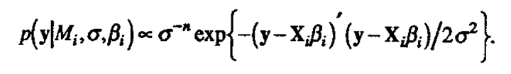
The elements of β_i are assigned independent prior normal distributions with mean 0 and variance γ²σ² (A priori ignorance of the direction of any particular effect is represented by the zero mean; the magnitude of the effect relative to experimental noise is thus captured through the parameter γ.) A noninformative prior distribution is employed for the overall mean β₀ and log(σ) so that p(β₀,σ) ^oc 1/σ where the likelihood is appreciable and negligible elsewhere. Having observed the data vector y, the posterior probability of the model M_i can then be written

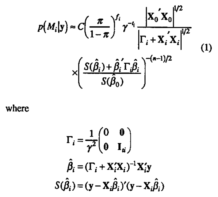
C is the normalization constant which forces all probabilities to sum to one and I_ti. is the t_i × t_i identity matrix. See the Appendix for further details of the derivation of (1).

The probabilities p(M_i |y) can be accumulated to compute the marginal posterior probability P_j that Factor j is active

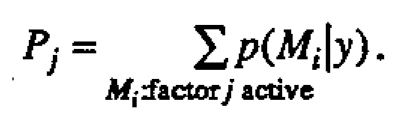
The probability P_j is just the sum of the posterior probabilities of all the distinct models in which the factor j is active. The probabilities {P_j} are thus calculated by direct enumeration over the 2^k possible models M_i. A large value for P would indicate that the factor j was active, and similarly, a value of P_j close to zero would indicate that the factor j was inert. After examining the {P_j}, the individual probabilities p(M_i |y) may further identify specific combinations of factors that are most likely active. We illustrate with some examples in the following section.

Examples

The analysis is demonstrated in this section on three examples which will help to show its utility. The first two examples illustrate its benefits for nongeometric Plackett-Burman designs. The remaining example demonstrates its application for designs, highlighting the issue of follow-up experiments for resolving ambiguities. In each example the posterior probabilities are computed with nominal value for π of 0.25 and y chosen to minimize the probability of no active factors. (The theoretical justification for this is given in the Appendix.) In practice, one might try different values of these parameters to gage sensitivity (see, for example, Box and Meyer (1986a)), but for the sake of brevity, that will not be done here. We will comment further on the effect of choice of parameters in the Discussion.

Example 1

In this example we illustrate some of the difficulties which may be encountered when analyzing the results of a nongeometric Plackett-Burman design and how the Bayesian analysis can help to overcome these difficulties. To aid further in illustrating and Understanding the concepts involved, this example was constructed by extracting 12 runs from the 2 reactor example from Box, Hunter and Hunter (1978)

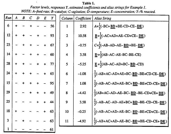
p. 376. Letters rather than numbers have been used to identify the experimental factors. The 12 runs chosen were those that would have been run if the first five columns of the 12-run Plackett-Burman array had been employed as a screening design for these five factors. The 12 runs are shown in Table 1. The run numbers shown are those from the original set of 32. Analysis of the full data set, as shown in Box, Hunter and Hunter (1978) showed main effects B, D and E, as well as the BD and DE interactions, were important.

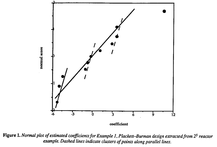
The 11 estimated effects, one for each column of the full Plackett-Burman design array, are shown in Table 1, and the normal plot of effects is shown in Figure 1. Only the main effect of factor B, catalyst level, clearly stands out. The other notable features of this plot are the gaps between groups of points falling along distinct parallel lines as illustrated in Figure 1. Daniel (1976) proposed that this indicates the possibility of outliers among the original observations (see also Box and Draper (1987), p. 131). If a particular outlying observation is biased by, say, a positive (negative) amount, then contrasts in which the observation enters positively (negatively) are shifted to the right and contrasts in which the observation enters negatively (positively) are shifted to the left. Thus the observation, if it exists, which enters positively (negatively) in the positive contrasts and negatively (positively) in the negative contrasts is identified as a potential outlier. Following this method, however, does not reveal any of the observations as clearly discordant.

The confounding structure of the Plackett-Burman design suggests another explanation for the unusual normal plot. As mentioned previously, the main effect of each factor is confounded with all two-factor interactions not involving that factor. Table 1 gives the alias relationships. The BD and DE interactions, which are known to be large from the full data analysis, are underlined. Taking into account the signs of the large interaction effects (the BD interaction is positive, the DE interaction is negative) reveals that column contrasts 1, 8, 9 and 11 are affected most. Contrasts 1 and 9 are shifted positively by the presence of these interactions and Contrasts 8 and 11 are shifted negatively. Other contrasts are affected to a lesser extent. This has the net effect of creating the unusual pattern of points in the normal plot and obscuring the identity of what are known, from the complete 2⁵, to be important factors.

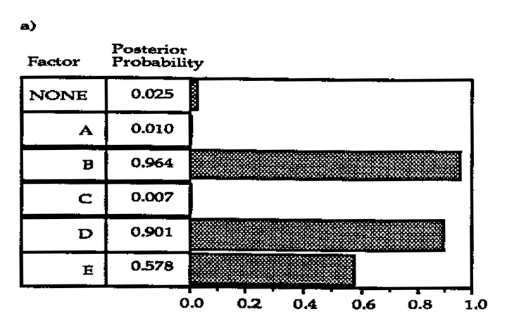
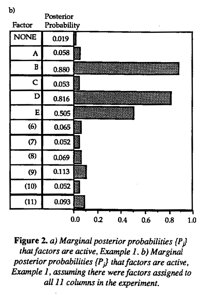
The Bayesian analysis was carried out on these data allowing for the possibility of two and three- factor interactions. The marginal posterior probabilities {P_j} are given in Figure 2a.. The results quite clearly identify factors B, D and E as active, and this is in agreement with the factors identified by analysis of the full 2⁵, Had this 12-run design been the one actually carried out the logical next step would be to fit the model involving factors B, D and E and their interactions to the data and do further analysis to determine if the effects were estimated with satisfactory precision. Additional runs might be indicated depending upon the objectives of the experiment.

This example has clearly shown that analyzing the data using the Bayesian model, which allows explicitly for the presence of interactions, can identify plausible explanations missed by conventional analysis. Two factors D and E, not originally picked up through the examination of the set of orthogonal column contrasts, were identified as active. The implications are apparent. One can imagine the negative impact of overlooking important factors at the screening stage of an experimental investigation. Given the experience of this example of studying only five factors in 12 runs, one can also imagine the difficulties created by the presence of interactions when up to 11 factors are screened with the 12-run Plackett-Burman array. To demonstrate that the Bayesian analysis would still be effective in the saturated case, the analysis was repeated pretending there had been 11 factors studied in this experiment. That is, for the sake of illustration, dummy factors (6) through (11) were assigned to the remaining columns of the Plackett-Burman array, and the Bayesian analysis repeated as though the design were saturated. The (P_j) are given in Figure 2(b), and the same three factors B, D and E are identified as active.

Example 2

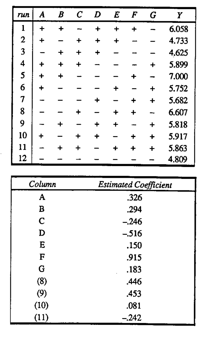
A 12-run Plackett-Burman design was employed to study fatigue life of weld repaired castings (Hunter, Hodi and Eager (1982)). (The possible presence of an interaction in this example was shown by Hamada and Wu (1991).) Seven factors were varied in this experiment. The design matrix, data, estimated effects and normal plot of effects are given in Figure 3. The normal plot rather dubiously supports the original authors' conclusion that factor F and possibly factor D had significant main effects. The plot also displays to some extent the behavior noted in the previous example, gaps among the points that indicate the possibility of interaction for a Plackett-Burman design.

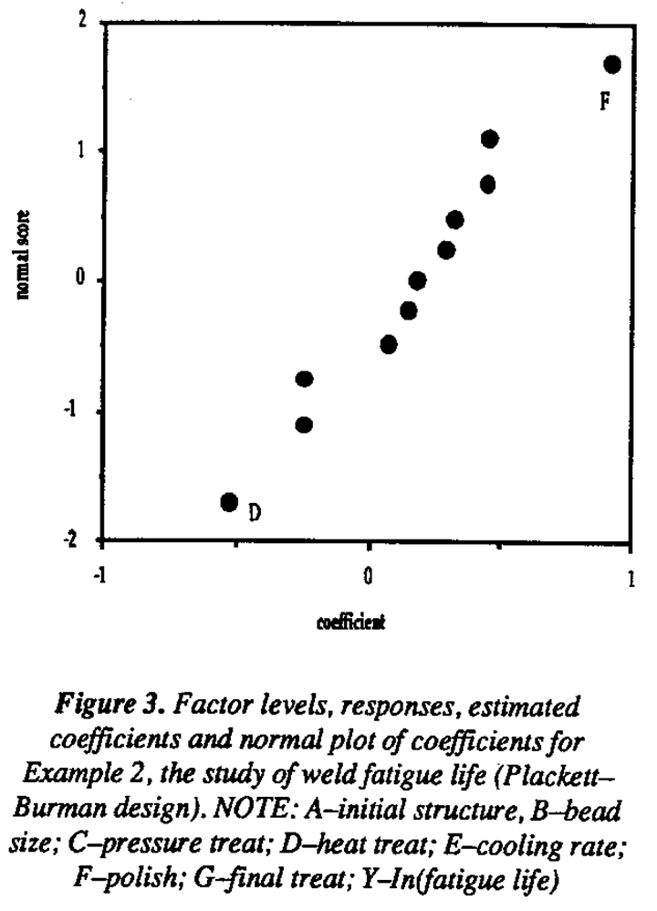
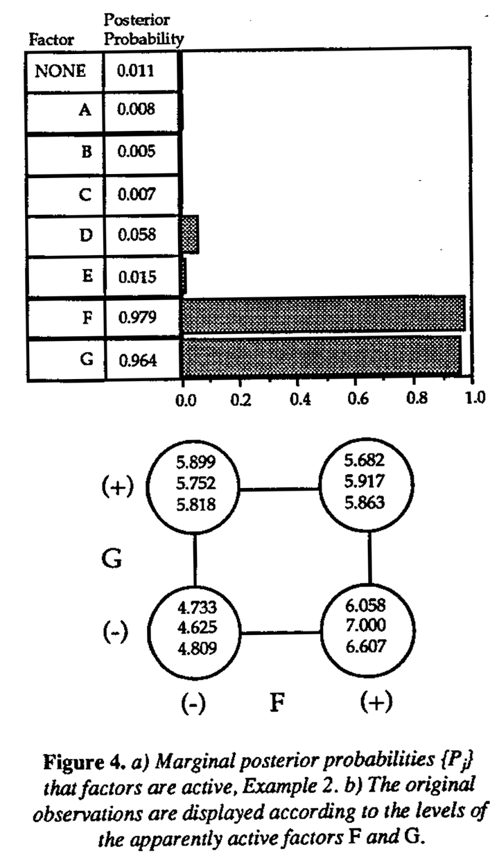
The Bayesian analysis was carried out on these data and the results are shown in Figure 4a. Factors F and G are identified as the active factors in this experiment with posterior probabilities of 0.979 and 0.964 respectively. On the right in Figure 4 the data are arranged according to the levels of factors F and G. It is clear from this display that a very plausible explanation for the data is the joint effect of these two factors. Because it has a small main effect, factor G was not flagged in the normal plot of effects. As in the previous example, interactions were camouflaged. This example verifies that in actual experiments conducted using Plackett-Burman nongeometric important effects involving interactions have probably been missed.

Example 3

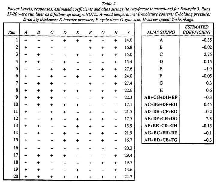
The third example is the 2^8-4 injection molding, example from Box, Hunter and Hunter (1978), p. 398. The design matrix, observed data, estimated effects and their alias strings (up to two-factor interactions) are given in Table 2. The normal plot of effects in Box, Hunter and Hunter (1978) showed that contrasts corresponding to effects C, E and AE+BF+CH+DG were too large to be explained by noise. There was also weak evidence to suggest the effect H might also be important. Box, et al., suggested that it was most likely either the AE or CH interaction which would explain the large contrast associated with AE+BF+CH+DG because these involved variables with large main effects. Factors A, C, E and H were thus identified in the original analysis as the potentially active factors in this experiment.

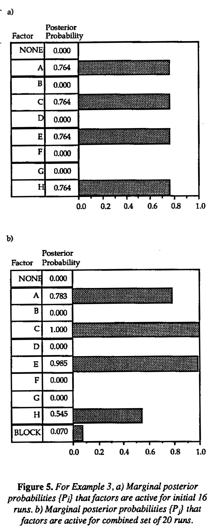
The marginal posterior probabilities {P_j} for each factor are displayed in Figure 5, again allowing for two and three-factor interactions. Factors A, C, E and H have marginal posterior probabilities of approximately 0.76 and thus clearly stand out as potentially active. These are the same four factors identified by the previous analysis. The remaining factors have essentially zero probability.

The 2^8-4 collapses to a replicated 2^4-1 design (Resolution IV) in these four factors, so it is not possible to obtain separate estimates of their main effects and interactions from the original 16 runs. Additional runs are required. Box, Hunter and Hunter (1978) Appendix 12B, described a four-run follow up design, runs 17-20 of Table 2 additional four runs were selected in order to obtain separate estimates of the AE, BF, CH and DG interactions as well as the block effect between runs 1-16 and runs 17-20. The assumption was made that no three-factor interactions were present. Solving a system of five equations in five unknowns, the AE+BF+CH+DG alias string was apparently resolved and CH identified as the large interaction. Factors C, E, and H were thus identified as the active factors for this experiment.

We reconsider the problem of setting up the follow-up design based on three concerns:

1. The Bayesian analysis indicated that factors B, D, F and G were very likely inert; was it necessary to obtain estimates of the BF and DG interactions from the follow-up design?
2. Should there be more concern about the possibility of three-factor interactions among the potentially active factors A, C, E, and H?
3. Should there be more concern for obtaining separate estimates of the other confounded factor interactions among the potentially active factors A, C, E, and H even though the contrasts associated with them were small?

The posterior probabilities were recomputed (Figure 5(b)) using the combined 20 runs, defining a ninth factor to be the block effect between the first 16 runs and the last four. All four factors A, C, E and H still stand out as potentially active. This is quite different from the conclusions drawn earlier by Box, Hunter and Hunter when factor A was judged to be inert after the follow-up experiment. The difference in the two analyses is the implicit assumption made by Box, Hunter and Hunter that three-factor interactions were not involved in the explanation of these data. They ruled out the possibility that the large contrast associated with the C main effect could have been the AEH interaction, the contrast associated with the H main effect could have been the ACE interaction, and so forth. (When the posterior probabilities are recomputed allowing for only two- factor interactions (not shown), Factors C, E and H have probabilities close to 1.0 and Factor A's probability is closer to 0.0.).

An alternative approach for setting up the follow-up design would be to assume that factors A, C, E, and H were the potentially active factors upon completion of the 16-run initial experiment. The design collapses to a half-fraction of the full factorial in these factors with defining relation I = ACEH. Running the other half fraction I = (-ACEH), an eight-run design, would allow estimation of all main effects, two and three-factor interactions involving A, C, E, and H, and confound the four-factor interaction with the block effect. The remaining four factors B, D, F, and G, assumed inert, would be set at some convenient levels within their ranges in the original design.

In general, it seems reasonable, and we tentatively recommend, that when a subset of the original set of experimental factors is identified as potentially active via the Bayesian analysis, the design of follow-up experiments to resolve ambiguities should focus on these factors.

Discussion

At the initial stage of a scientific investigation, emphasis is on the model identification stage of the iterative problem-solving process (see, for example, Box and Jenkins (1976)). Screening designs are employed in these situations to identify various hypotheses (models) that may be explored in subsequent experiments. Alternative possibilities are tentatively entertained until confirmatory data allows further model discrimination and refinement. It is important to attempt to identify all plausible explanations of the data obtained in a screening experiment and not overlook potentially important factors. The Bayesian analysis proposed here considers a broad, though not exhaustive, class of models, evaluating each member of the class in light of the observed data. Other models which bear consideration are, for example, those concerning dispersion effects (Box and Meyer (1986b)) and outliers (Box and Meyer (1987)).

Visual displays of the data are, in general, known to be effective in stimulating the creative process of model identification. The graphical methods employed may involve plotting of the "raw" data, e.g. scatter plots and scatter-plot matrices. Other methods involve plotting of statistics, suggested by the class of models being considered, which summarize features of the data useful for model identification. In this category are, for example, plots of the lagged autocorrelation and partial autocorrelation in time-series analysis. The plotting of the marginal posterior probabilities described here is in this latter class of model-identification tools. In some cases, a model identified via the posterior probabilities can be fit using accepted estimation methods. More often additional experiments will be run before one model is (tentatively) identified and estimated.

In any visual display of data, particularly during model identification, one seeks patterns that may suggest new and interesting hypotheses not yet considered. It is in this spirit that the marginal posterior probabilities {P_j} should be considered. The absolute magnitudes of the probabilities are less important than the pattern of probabilities and their relative magnitudes. Probabilities which stand out from the others, even if they are less than 1/2, identify factors or models worthy of further consideration. In practice there is no harm done in interpreting the posterior probabilities liberally. Usually an additional experiment or experiments will be run to identify with some certainty the factors that matter and the nature of their effects. The examples of the previous section illustrate how this might work in practice.

The Bayesian approach requires specification of prior distributions and parameters of those distributions. The choice of noninformative prior distributions for the parameters βο and σ is a standard one, and the interested reader is referred to Box and Tiao (1973) for further Discussion. The choice of normal prior distribution N(0, γ²σ²) for remaining elements of Bi is a natural one because

1. it is an informative and conjugate prior distribution, leading to mathematical tractability;
2. there is typically prior ignorance of the direction of any particular effect, leading to the zero mean;
3. important main effects and interactions tend, in our experience, to be of roughly the same order of magnitude, justifying the parsimonious choice of one common scale parameter g; uncertainty in g can be handled as described in the Appendix.

The prior probability π must also be specified. Increasing p tends to increase all of the {P_j} but usually has little effect on which probabilities stand out from the rest. The nominal choice of π = 0.25 has served well in our experience, but the individual experimenter should choose a value of pi that represents his prior expectation of the proportion of active factors. The analysis can also be repeated for a few different values of π, say 0.1, 0.25 and 0.5 and the results compared. Usually the same factors will be identified as potentially active, but if not, it is important to remember the ultimate purpose, which is to identify different plausible models which may be explored further through model-fitting and additional experiments.

The approach we have developed is completely general and can be useful for any experiment where confounding and fractionation make results difficult to interpret. Other irregularities, such as when data are missing, extra data are available, factor settings for certain runs have deviated from those originally designed, and so on, have traditionally led to problems analyzing results. We have found the Bayesian model identification scheme to be very helpful for sorting out potentially active factors in these situations as well, and we are continuing to investigate these areas. Determining follow-up designs for further model discrimination may be facilitated by the Bayesian framework (see Example 3), and we are investigating this as well.

The computations for the examples were carried out in Fortran on an IBM 3090 300E mainframe computer, rated at 45 mips. Computation time is roughly proportional to 2k for a design with k factors.

Conclusions

Testing several factors in only a handful of runs in a fractionated screening experiment usually results in more than one plausible explanation for the data. This is where the economy of fractional factorial designs is valuable: the number of plausible hypotheses can be reduced at each round of experimentation with far fewer total runs than one supposedly comprehensive experiment. By including more variables in the screening experiment, arbitrarily eliminating variables at the outset of an investigation is also avoided.

Interpreting the results from these screening experiments can be a difficult task. This is particularly true of nongeometric Plackett-Burman designs which have been shown to be difficult to interpret in the presence of interactions. Interactions are hidden in the normal plot of effects (or any other method based on the orthogonal column contrasts) and important factors can be completely overlooked. The Bayesian analysis proposed here can greatly facilitate the identification of active factors. All possible explanations of the data are considered, including interactions, and those which explain the data well are identified by their large posterior probabilities. We have shown in the examples that very plausible models, undiscovered through conventional analysis, were identified through our Bayesian method.

Acknowledgments

This research was sponsored by the Alfred P. Sloan Foundation, the United States Army under Contract No. DAAG29-80-C-0041, by the National Science Foundation Grant No. DMS-8420968, by the Vilas Trust of the University of Wisconsin-Madison, by The Lubrizol Corporation and aided by access to the research computer of the University of Wisconsin-Madison Statistics Department. The authors would like to thank Elizabeth Schiferl, Sara Pocinki, Robert Wilkinson and two referees for their helpful discussion and comments, and numerous colleagues for trying the method on real examples.

The Fortran program MBJQT92 for performing the computations described here is available at nominal cost from Scientific Computing Associates, Lincoln Center, Suite 106, 4513 Lincoln Avenue, Lisle, Illinois 60532, (708) 960-1698.

Appendix

Calculation of p(y|M_i)

The predictive density p(y|M_i)is obtained by the following integration:

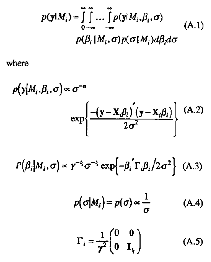
The above expressions (A.3) and (A.4), being noninformative in the overall mean β₀ and σ, are assumed to hold only in the region where the likelihood (A.2) is appreciable as a function of β₀ and u. Outside this region, however, it is assumed that the likelihood dominates the integrand in (A.1) and the expressions (A.3) and (A.4) can be used over the full range of integration.

Constants which force density functions to integrate to unity have been dropped for simplicity as they would cancel out eventually in the expression (1) for p(M_i|y).

Performing the integration with respect to β_i first

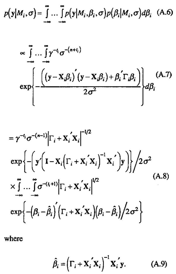
The expression inside the integral is proportional to the density of a multivariate normal distribution with mean and covariance matrix 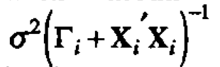and so integrates to a constant, leaving

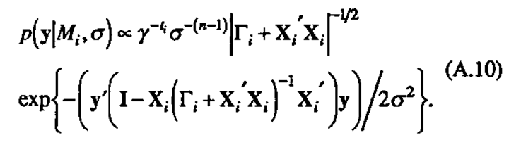
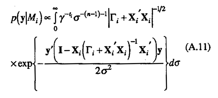
Now integrating against p(σ) to obtain p(y|M_i)

and making a change of variables

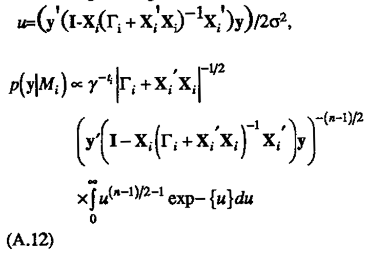
The latter integral is a gamma function (Γ((n-1)12)) and thus constant, leaving

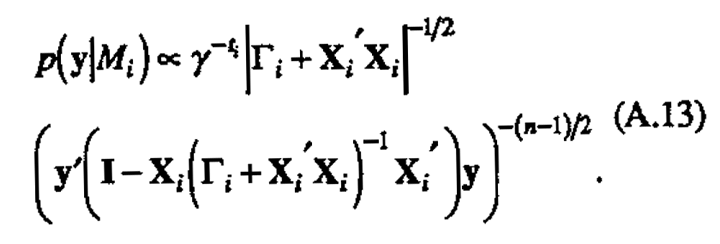
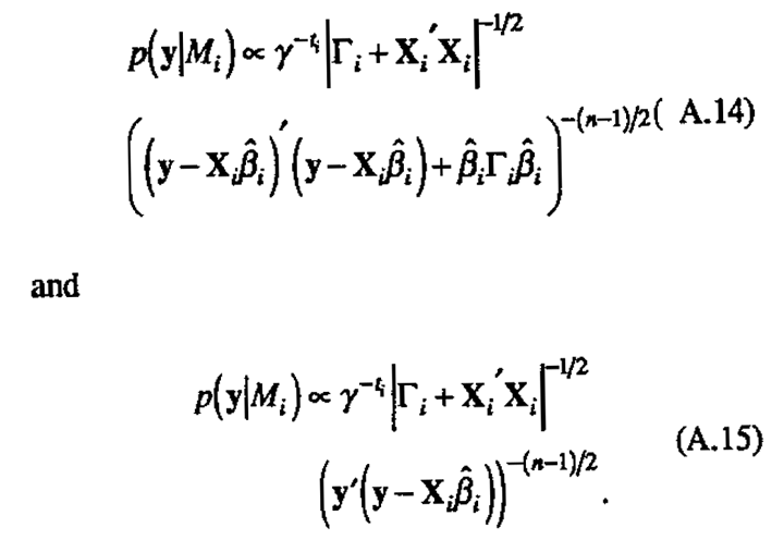
can be rewritten to give two equivalent forms for p(y|M_i)

Uncertainty in γ

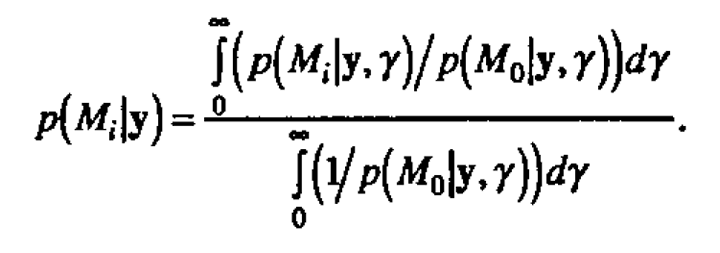
The full Bayesian solution for handling the unknown parameter γ is to specify its noninformative) prior distribution p(γ) and perform a further integration with respect to this would entail either obtaining the expression for p(γ) via an additional integration against p(γ) or integrating the expression for p(M_i|y,γ) against p(γ|y), to obtain an expression free of γ. A convenient approximation reasonable for purposes of model identification, is to evaluate p(M_i|y,γ) as the value y which maximizes the posterior density p(γ|y). Setting the prior density p(γ) to be locally uniform, the posterior density p(γ|y) is given approximately by

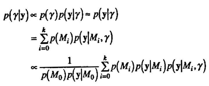
(because p(M₀)p(y|M₀) does not depend on γ).

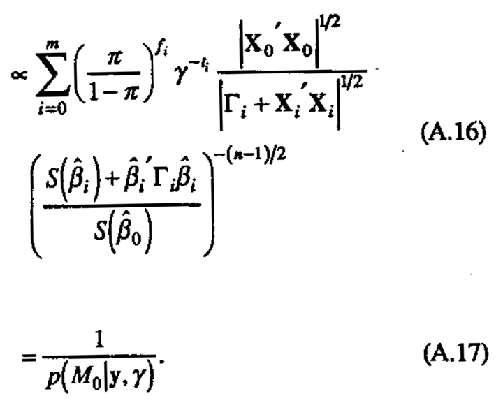
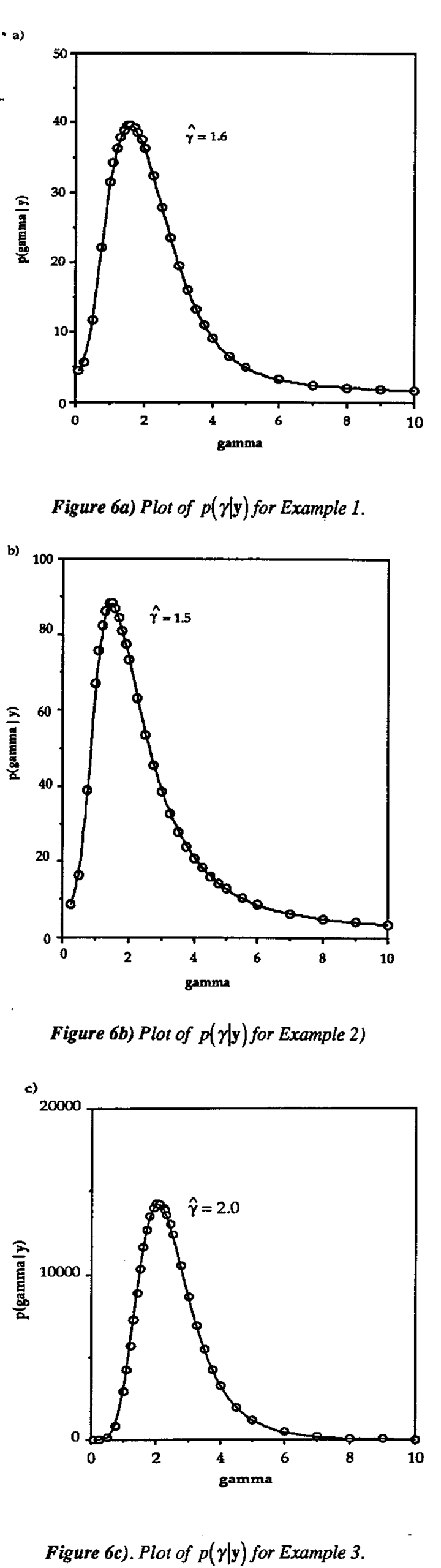
Thus the value which maximizes the posterior density (and likelihood) also minimizes the probability of no active factors. Evaluating p(M₀|y,γ) for this value of γ is intuitively appealing on the grounds that the data are interpreted from the approach that minimizes the chance of nothing interesting showing up. The (unscaled) posterior densities of γ for Examples 1-3 are given in Figure 6. In practice, we compute to the nearest tenth by repeating the posterior probability calculations for y between 0.5 and 5.0 in increments of 0.5, then in increments of 0.1 on the subinterval which surrounds the maximum found on the first iteration.

Two situations which may occur in practice that deserve further discussion are

1. two or more local maxima of p(γ|y): in this case we run the analysis for each value of y that gives a local maximum of p(γ|y) and compare results; models identified by any of the analyses are explored further through model-fitting and plotting;
2. no maxima of p(γ|y), which can monotonically increase or decrease: in this case we repeat the analysis for several values in the sensible range for γ, say 0.5 to 10.0, and compare results; again, models identified by any of the analyses are explored further through model-fitting and plotting.

The full Bayesian analysis can be carried out by numerically performing the integration

This is computationally a much more intensive task, and we prefer the approach of estimating γ or a repeating the analysis for various fixed γ and comparing results.

References

• Box, G. E. P. (1952). "Multi-factor Designs of First Order." Biometrika, 39. pp. 49-57.
• Box, G. E. P., and Draper, N. R. (1987). Empirical Model-Building and Response Surface. John Wiley & Sons; New York. Box, G.E.P. and Draper, N.R. (1986),
• Box, G. E. P., and Hunter, J. S. (1961). "The 2^k-p Fractional Factorial Designs." Technometrics, 3. pp. 311-351, 449-458.
• Box, G. E. P., Hunter, W. G., and Hunter, J. S. (1978). Statics for Experimenters. John Wiley & Sons; New York.
• Box, G. E. P., and Jenkins, G. (1976). Time Series Analysis: Forecasting and Control. Holden-Day; San Francisco.
• Box, G. E. P., and Meyer, R. D. (1986a). "An Analysis for Unreplicated Fractional Factorials: Optimal Multifactorial Experiments." Technometrics, 28. pp. 11-18.
• Box, G. E. P., and Meyer, R. D. (1986b). "Dispersion Effects From Fractional Designs." Technometrics, 28. pp. 19-27.
• Box, G. E. P., and Meyer, R. D. (1987). "Analysis of Unreplicated Factorials Allowing for Possibly Faulty Observations." in Design. Data and Analysis. C. Mallows (ed). John Wiley & Sons; New York.
• Box, G. E. P., and Tiao, G. C. (1968). "A Bayesian Approach to Some Outlier Problems." Biometrika, 55.pp. 119-129.
• Box, G. E. P., and Tiao, G. C. (1973). Bayesian Inference in Statistical Analysis. Addison Wesley; Reading, Massachusetts.
• Box, G. E. P., and Wilson, K. B. (1951). "On the Experimental Attainment of Optimum Conditions." J. Roy. Stat. Soc., Ser. B, 13. pp. 1-45.
• Daniel, C. (1959). "Use of Half-Normal Plots in Interpreting Factorial Two-Level Experiments." Technometrics, 1. pp. 311-341.
• Daniel, C. (1976). Applications of Statics to Industrial Experimentation. John Wiley & Sons; New York.
• Finney, D.J. (1945). "The Fractional Replication of Factorial Arrangements." Annals of Eugenics, 12. pp. 291-301.
• Hamada, M., and Wu, C. F. J. (1991). "Analysis of Designed Experiments With Complex Aliasing." IIQP Research Report RR-91-01. University of Waterloo, Waterloo, Ontario, Canada.
• Hunter, G.B., Hodi, F.S., and Eager T.W. (1982). "High-Cycle Fatigue of Weld Repaired Cast Ti.6A1-4V." Metallurgical Transactions 13A. Pp. 1589-1594
• Lenth, R.V. (1989). "Quick and Easy Analysis of Unreplicated Factorials." Technometrics, 31 pp. 469-473.
• Plackett, R. L., and Burman, J.P. (1946) "Design of Optimal Multifactorial Experiments." Biometrika, 23. pp. 305-325